19 Temporal filters
19.1 Introduction
Although adding time might seem like a trivial extension from 2D signals to 3D signals, and in many aspects it is, there are some properties of how the world behaves that make sequences different from arbitrary 3D signals. In 2D images, most objects are bounded, occupying compact and well-defined image regions. However, in sequences, objects do not appear and disappear instantaneously unless they get occluded behind other objects or enter or exit the scene through doors or the image boundaries. So, the behavior of objects across time \(t\) is very different than their behavior across space \(n,m\). In time, objects move and deform, defining continuous trajectories that have no beginning and never end.
19.2 Modeling sequences
Sequences will be represented as functions \(\ell (x,y,t)\), where \(x,y\) are the spatial coordinates and \(t\) is time. As before, when processing sequences, we will work with the discretized version that we will represent as \(\ell \left[n,m,t \right]\), where \(n,m\) are the pixel indices and \(t\) is the frame number. Discrete sequences will be bounded in space and time, and can be stored as arrays of size \(N \times M \times P\).
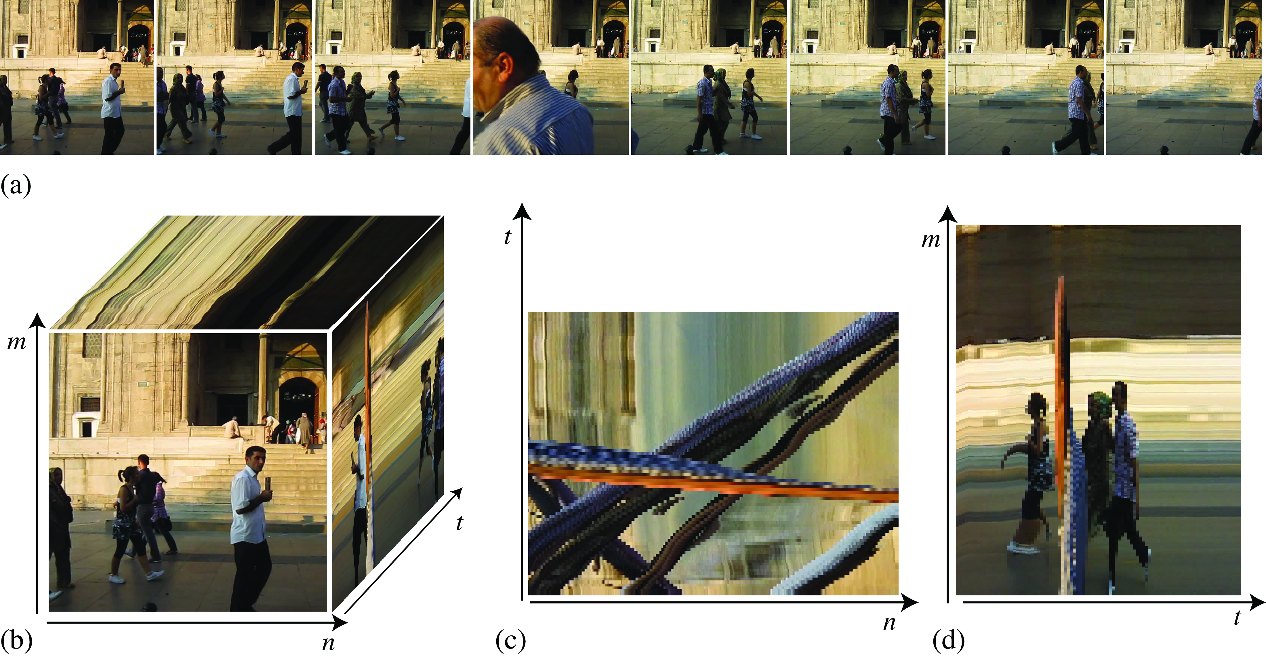
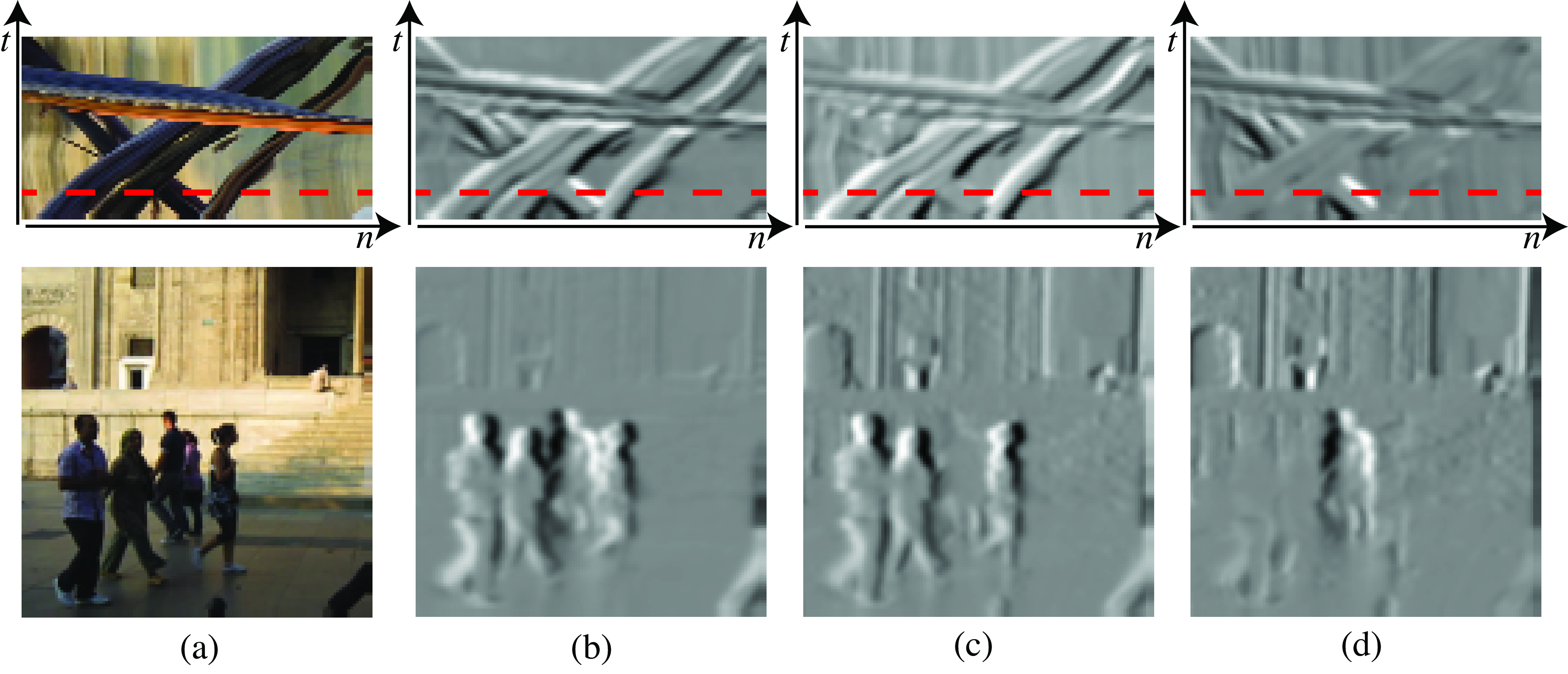
Figure 19.1 illustrates this with one sequence shown in Figure 19.1 (a). This sequence has 90 frames and shows people on the street walking parallel to the camera plane and at different distances from the camera. Figure 19.1 (b) shows the space-time array \(\ell \left[n,m,t \right]\). When we look at a picture, we are looking at a 2D section, \(t\)=constant, of this cube. But it is interesting to look at sections along other orientations. Figure 19.1 (c) and Figure 19.1 (d) show sections for \(m\)=constant and \(n\)=constant, respectively. Although they are also 2D images, their structure looks very different from the images we are used to seeing. Figure 19.1 (c) shows a horizontal section that is parallel to the direction of motion of the people walking. Here we see straight bands with different orientations. These bands appear to occlude each other. Each band corresponds to one person, and its orientation is given by the speed of walk and the direction of motion. Figure 19.1 (d) looks like a photo-finish photograph, similar to those used in sporting races. In both images (c) and (d), static objects appear as vertical stripes in (b) and horizontal stripes in (d).
One special sequence is when the image has a global motion with constant velocity \((v_x,v_y)\). In such a case, we can write: \[ \ell (x,y,t) = \ell _0 (x-v_xt,y-v_yt) \tag{19.1}\]
where \(\ell _0(x,y)= \ell (x,y,0)\) is the image being translated, and \(v_x\) and \(v_y\) are constants. At time \(t\) the image \(\ell _0(x,y)\) is translated by the vector \((v_x t, v_y t)\) as described by Equation 19.1. The pixel value at location \((x=0, y=0)\) at time \(t=0\) will appear at time \(T\) in location \((x=v_x T, y=v_y T)\). This is what we see in Figure 19.1 (c) where the bands are created by moving pixels.
We use continuous values for \(x\), \(y\), and \(t\), and continuous images, \(\ell _0(x,y)\), because it allows us to deal with any velocity values. This function also assumes that the brightness of the pixels does not change while the scene is moving (constant brightness assumption).
The constant brightness assumption is the initial hypothesis of most motion estimation algorithms. We will devote multiple chapters in Part Understanding Geometry to study motion in depth.
In general, sequences will be more complex, but the properties of a globally moving image are helpful to understand local properties in sequences. We can also write models for more complex sequences. For instance, a sequence containing a moving object over a static background can be written as: \[ \ell (x,y,t) = b(x,y) (1-m(x-v_xt,y-v_yt)) + o(x-v_xt,y-v_yt) m(x-v_x t,y-v_y t) \] where \(b(x,y)\) is the static background image, \(o(x,y)\) is the object image moving with speed \((v_x,v_y)\), and \(m(x,y)\) is a binary mask that moves with the object and that models the fact that the object occludes the background.
19.3 Modeling sequences in the Fourier domain
The FT of a globally moving image is (using the shift property): \[ \mathscr{L} (w_x,w_y,w_t) = \mathscr{L}_0 (w_x, w_y) \delta (w_t + v_x w_x + v_y w_y) \] The continuous FT of the sequence is equal to the product of the 2D FT of the static image \(\ell _0(x,y)\) and a delta wall. To better understand this function, let’s look at a simple example in only one spatial dimension, as shown in Figure 19.2.
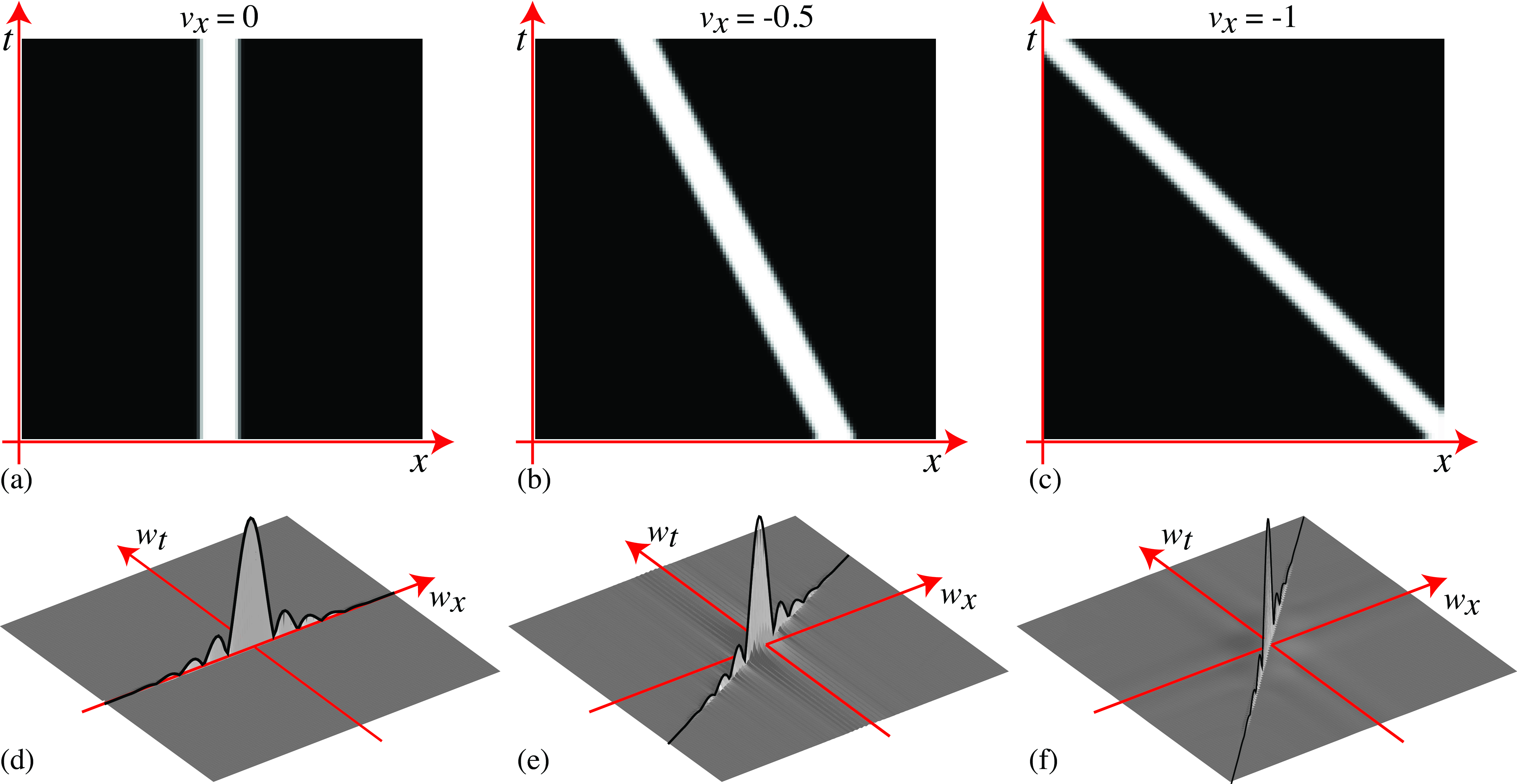
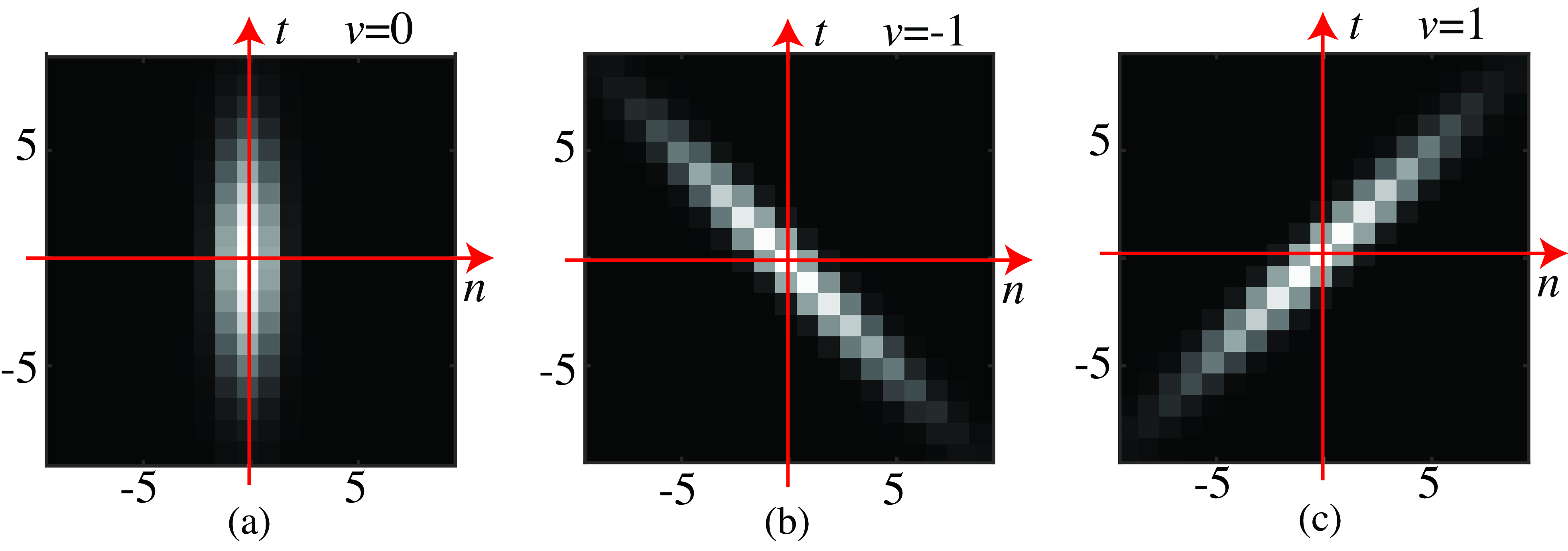
Figure 19.2 shows the FT for a sequence with one spatial dimension, \(\ell (x,t)\), that contains a blurry rectangular pulse moving at three different speeds towards the left. Figure 19.2 (a) shows a sequence when the pulse is static, and Figure 19.2 (d) shows its FT. Across the spatial frequency \(w_x\), the FT is approximately a sinc function.
Across the temporal frequency \(w_t\), as the signal is constant, its FT is a delta function. Therefore, the FT is a sinc function contained inside a delta wall in the line \(w_t=0\). Figure 19.2 (b) shows the same rectangular pulse moving towards the left, \(v_x=0.5\). Figure 19.2 (e) shows the sinc function but skewed along the frequency line \(w_t+0.5w_x=0\). Note that this is not a rotation of the sinc function from Figure 19.2 (d) as the locations of the zeros lie at the same \(w_x\) locations. Figure 19.2 (c) shows the pulse moving at a faster speed resulting in a larger skewing of its FT, Figure 19.2 (f).
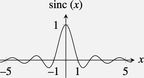
The sinc function is the FT of a box kernel. In the continuous domain, the sinc function has the form: \[ \text{sinc}(x) = \frac{\sin (\pi x)}{\pi x} \] This function has its maximum at \(x=0\) and then has decreasing oscillations.
We will discuss this further in Section 20.4.1.
19.4 Temporal filters
Linear spatio-temporal filters can be written as spatio-temporal convolutions between the input sequence and a convolutional kernel (impulse response). Discrete spatiotemporal filters have an impulse response \(h \left[n,m,t \right]\). The extension from 2D filters to spatio-temporal filters does not have any additional complications. We can also classify filters as low-pass, high-pass, etc. But in the case of time, there is another attribute used to characterize filters: causality.
- Causal filters: These are filters with output variations that only depend on the past values of the input. This puts the following constraint: \(h \left[n,m,t \right]=0\) for all \(t<0\). This means that if the input is an impulse at \(t=0\), the output will only have non-zero values for \(t>0\). If this condition is satisfied, then the filter output will only depend on the input’s past for all possible inputs.
- Non-causal filters: When the output has a dependency on future inputs.
- Anti-causal filters: This is the opposite, when the output only depends on the future: \(h \left[n,m,t \right]=0\) for all \(t>0\).
Many filters are non-causal and have both causal and anti-causal components (e.g., a Gaussian filter). Note that non-causal filters cannot be implemented in practice and, therefore, any filter with an anti-causal component will have to be approximated by a purely causal filter by bounding the temporal support and shifting in time the impulse response.
In this chapter, we have written all the filters as convolutions. However, some filters are better described as difference equations (this is especially important in time). An example of a difference equation is: \[ \ell _{out} \left[n,m,t \right] = \ell _{in} \left[n,m,t \right] + \alpha \, \ell _{out} \left[n,m,t-1 \right] \] where the output \(g\) at time \(t\) depends on the input at time \(t\) and the output at the previous time instant \(t-1\) multiplied by a constant \(\alpha\). We can easily evaluate the impulse response, \(h \left[n,m,t \right]\), of such a filter by replacing \(\ell \left[n,m,t \right]\) with an impulse, \(\delta \left[n,m,t \right]\). The impulse response is: \[ h \left[n,m,t \right] = \alpha^t \delta \left[n,m \right] u \left[t \right] \] where \(u\left[t \right]\), called the Heaviside step function, is: \[ u \left[t \right] = \begin{cases} 0 & \quad \text{if } t <0 \\ 1 & \quad \text{otherwise }\\ \end{cases} \]
The Heaviside step function, \(u \left[t\right]\), is an infinite length function with the form
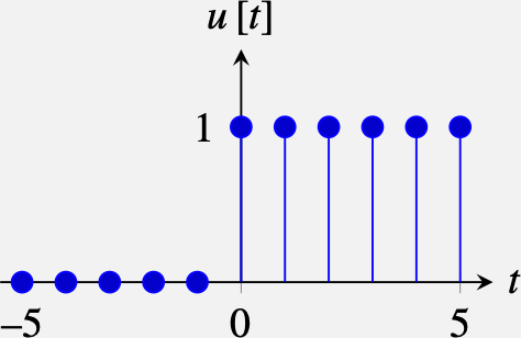
Most filters described by difference equations have an impulse response with infinite support. They are called IIR (Infinite Impulse Response) filters. IIR filters can be further classified as stable and unstable. Stable filters are the ones that given a bounded input, \(| \ell _{in} \left[n,m,t \right] |<A\), produce a bounded output, \(| \ell _{out} \left[n,m,t \right] | <B\). For this to happen, the impulse response has to be bounded. In unstable filters, the amplitude of the impulse response diverges to infinity. In the previous example, the filter is stable if and only if \(| \alpha | < 1\).
Let’s now describe some spatio-temporal filters.
19.4.1 Spatiotemporal Gaussian
As with the spatial case, we can define the same low-pass filters: the box filter, triangular filters, etc. As an example, let’s focus on the Gaussian filter. The spatio-temporal Gaussian is a trivial extension of the spatial Gaussian filter we have seen in @sec-spt_gaussian: \[ g(x,y,t; \sigma_x,\sigma_t) = \frac{1}{(2 \pi)^{3/2} \sigma_x^2\sigma_t} \exp{-\frac{x^2 + y^2}{2 \sigma_x^2}} \exp{-\frac{t^2}{2 \sigma_t^2}} \tag{19.2}\]
Where \(\sigma_x\) is the width of the Gaussian along the two spatial dimensions, and \(\sigma_t\) is the width in the temporal domain. As the units for \(t\) and \(x,y\) are unrelated, it does not make sense to set all the \(\sigma\)s to have the same value.
We can discretize the continuous Gaussian by taking samples and building a 3D convolutional kernel. We can also use the binomial approximation. The 3D Gaussian is separable, so it can be implemented efficiently as a convolutional cascade of 3 one-dimensional kernels. Figure 19.3 (a) shows a spatio-temporal Gaussian. The temporal Gaussian is a non-causal filter; therefore, it is not physically realizable. This is not a problem when processing a video stored in memory. However, if we are processing a streamed video, we will have to bound and shift the filter to make it causal, which will result in a delay in the output.
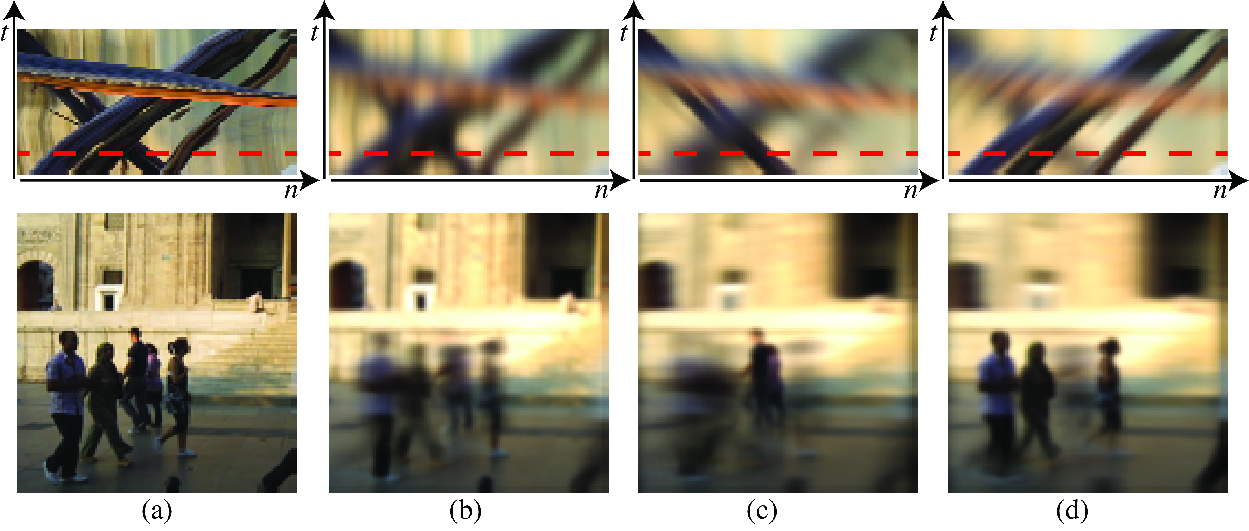
Figure 19.4 (a) shows one sequence, and Figure 19.4 (b) shows the sequence filtered with the Gaussian from Figure 19.3 (a). This Gaussian has a small spatial width, \(\sigma=1\), and a large temporal width, \(\sigma_t=4\), so the sequence is strongly blurred across time. The moving objects show motion blur and are strongly affected by the temporal blur, while the static background is only affected by the spatial width of the Gaussian.
How could we create a filter that keeps sharp objects that move at some velocity \((v_x,v_y)\) while blurring the rest? Figure 19.4(c) shows the desired output of such a filter. The bottom image shows one frame for a sequence filtered with a kernel that keeps sharp objects moving left at 1 pixel/frame while blurring the rest. This filter can be obtained by skewing the Gaussian: \[ g_{v_x,v_y}(x,y,t) = g(x - v_xt,y - v_yt, t) \] This directional blur is not a rotation of the original Gaussian as the change of variables is not unitary, but the same effect could be obtained with a rotation. Figure 19.4(c) shows the effect when \(v_x=-1, v_y=0\). The Gaussian is shown in Figure 19.3(b). The space-time section shows how the sequence is blurred everywhere except one oriented band corresponding to the person walking left. Figure 19.4(d) shows the effect when \(v_x=1, v_y=0\). The output of this filter looks as if the camera was tracking one of the objects while the shutter was open, producing a blurry image of all the other objects.
19.4.2 Temporal derivatives
Spatial derivatives were useful to find regions of image variation such as object boundaries. Temporal derivatives can be used to locate moving objects. We can approximate a temporal derivative for discrete signals as: \[ \ell \left[m,n,t\right] - \ell \left[m,n,t-1\right] \]
When implementing temporal filters it is important to use causal filters. A causal filter depends only on the present and past input samples.
As in the spatial case, it is useful to compute temporal derivatives of spatio-temporal Gaussians: \[ \frac{\partial g}{\partial t} = \frac{-t}{\sigma_t^2} g(x,y,t) \] where \(g(x,y,t)\) is the Gaussian as written in Equation 19.2. We can compute the spatio-temporal gradient of a Gaussian: \[ \nabla g = \left( g_x(x,y,t), g_y(x,y,t), g_t(x,y,t) \right) = \left(-x/\sigma^2, -y/\sigma^2, -t/\sigma_t^2 \right) g(x,y,t) \tag{19.3}\] We can use the analytic form of the spatiotemporal Gaussian derivatives from Equation 19.3 to discretize the filter, by taking samples at discrete locations in space and time, and use the resulting discrete spatiotemporal kernel to filter an input discrete sequence. These filters can be used for many applications. Let’s look at one practical example: What should we do if we want to remove only the objects moving at a particular velocity?
To answer that question, we will first assume the sequence contains a single object moving at a constant velocity. We will then compute the derivatives along \(x\), \(y\), and \(t\) of the sequence and we will find out what particular linear combination of those derivatives makes the output go to zero only when the input sequence moves at a target velocity.
In the case of a moving image with velocity \((v_x, v_y)\), the sequence is \[ \ell (x,y,t) = \ell _0 (x-v_xt,y-v_yt) \tag{19.4}\] We can compute the temporal derivative of \(f(x,y,t)\) as: \[ \frac{\partial \ell}{\partial t} = \frac{\partial \ell _0}{\partial t} = -v_x \frac{\partial \ell _0}{\partial x} - v_y \frac{\partial f_0}{\partial y} \tag{19.5}\]
This result is interesting because it shows that for a moving image there is a relationship between the temporal derivative of the sequence and the spatial derivatives a long the direction of motion. We can use this relationship to find a linear combination of the temporal and spatial derivatives so that the output is zero.
In fact, if we compute the gradient of the Gaussian along the vector \(\left[1,v_x,v_y\right]\):
\[ h(x,y,t;v_x,v_y) = g_t+v_xg_x+v_yg_y = \nabla g \left( 1,v_x,v_y \right)^\top \tag{19.6}\]
we get a kernel \(h(x,y,t;v_x,v_y)\) that we can use as a spatiotemporal filter that will do exactly what we were looking for. Indeed, if we convolve it with the input sequence \(\text{img}_0 (x-v_x t,y-v_y t)\) we get a zero output (using Equation 19.5):
\[ \begin{split} \ell _0 (x-v_x t, y-v_y t) \circ h & = \ell _0 (x-v_x t, y-v_y t) \circ \left( g_t + v_x g_x + v_y g_y \right) \\ & = \left( \frac{\partial \ell _0}{\partial t} + v_x \frac{\partial \ell _0}{\partial x} + v_y \frac{\partial \ell _0}{\partial y} \right) \circ g \\ & = 0 \end{split} \]
The filter \(h\) from Equation 19.6 is shown in Figure 19.5. As this filter is 3D, we show it as a sequence for different velocities. Each row in the figure corresponds to one particular velocity \(v_x, v_y\). In the example shown in Figure 19.5 (a), the Gaussian has a width of \(\sigma^2=\sigma_t^2=1.5\) and has been discretized as a 3D array of size \(7 \times 7 \times 7\). Figures Figure 19.5 (b, c, and d) show the filter \(h\) for different velocities: \((v_x, v_y) = (0,0)\), \((1,0)\), and \((-1,0)\).
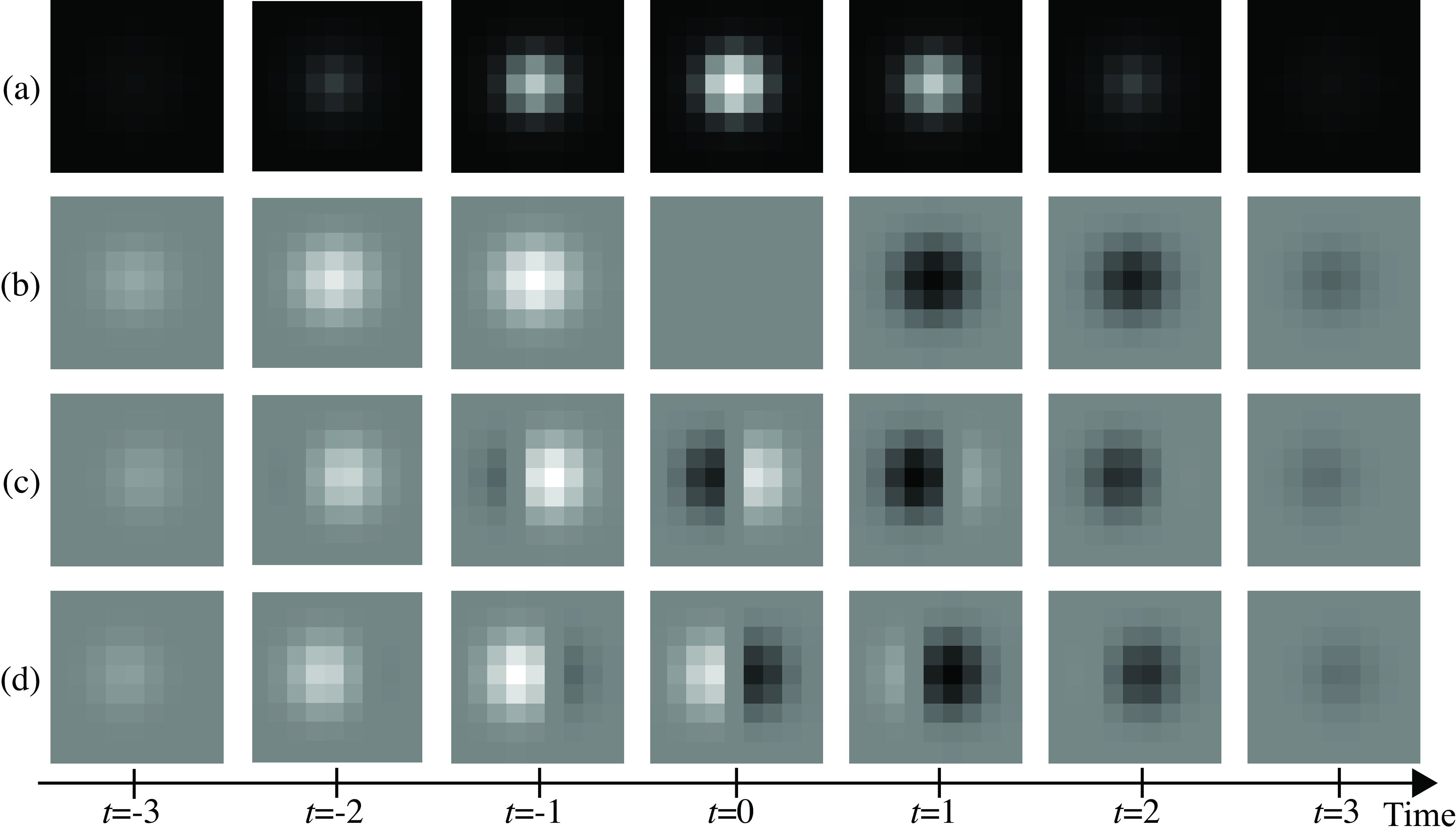
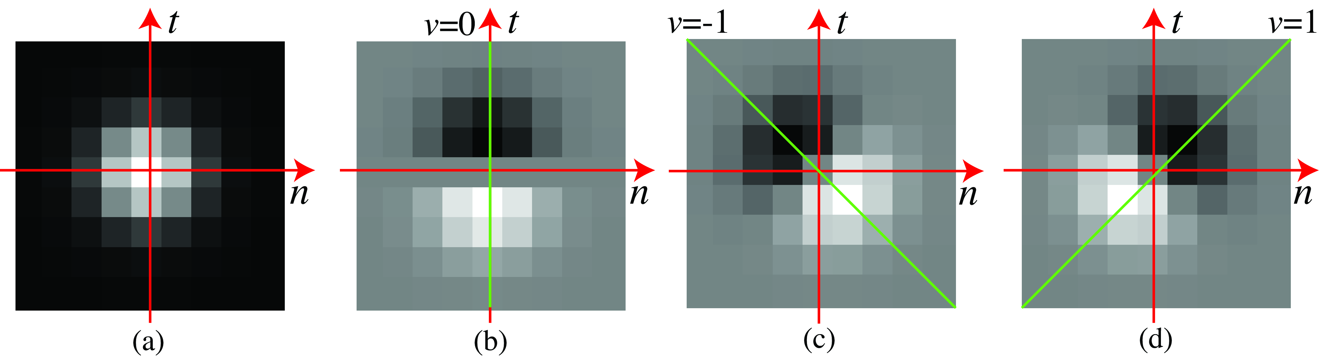
Figure 19.6 shows a different visualization of the same filter \(h\) from Equation 19.6. Each image in Figure 19.6 shows a space-time section of the same spatiotemporal Gaussian derivatives as the ones shown in Figure 19.5. Both visualizations are equivalent and help to understand how the filter works.
Such a filter \(h\) will cancel any objects moving at the velocity \((v_x,v_y)\). By using different filters, each one computing derivatives along different space-time orientations, we can create output sequences where specific objects disappear, as shown in Figure 19.7. This filter is called a nulling filter [1].
Note that despite assuming that the sequence contained a single moving object when deriving the formulation for the nulling filter, the filter also works in sequences with multiple objects moving at different speeds, as shown in Figure 19.7. This is because the operations are local (the kernel \(h\) has a small size), and the behavior will be correct if in a local image patch there is only one velocity present. In fact, it is easy to show that the method will also work if the sequence is a sum of several moving transparent layers.
19.5 Concluding Remarks
In this chapter, we have discussed different types of spatiotemporal filters used to analyze video. However, we have not presented how these filters can be used to estimate useful quantities such as velocity. We will devote several chapters in Part Understanding Motion to motion estimation.