24 Convolutional Neural Nets
24.1 Introduction
The neural nets we saw in Chapter 12 are designed to process generic data. But in many domains, the data has special structure, and we can design neural net architectures that are better suited to exploiting that structure. Convolutional neural nets, also called convnets or CNNs, are a neural net architecture especially suited to the structure in visual signals.
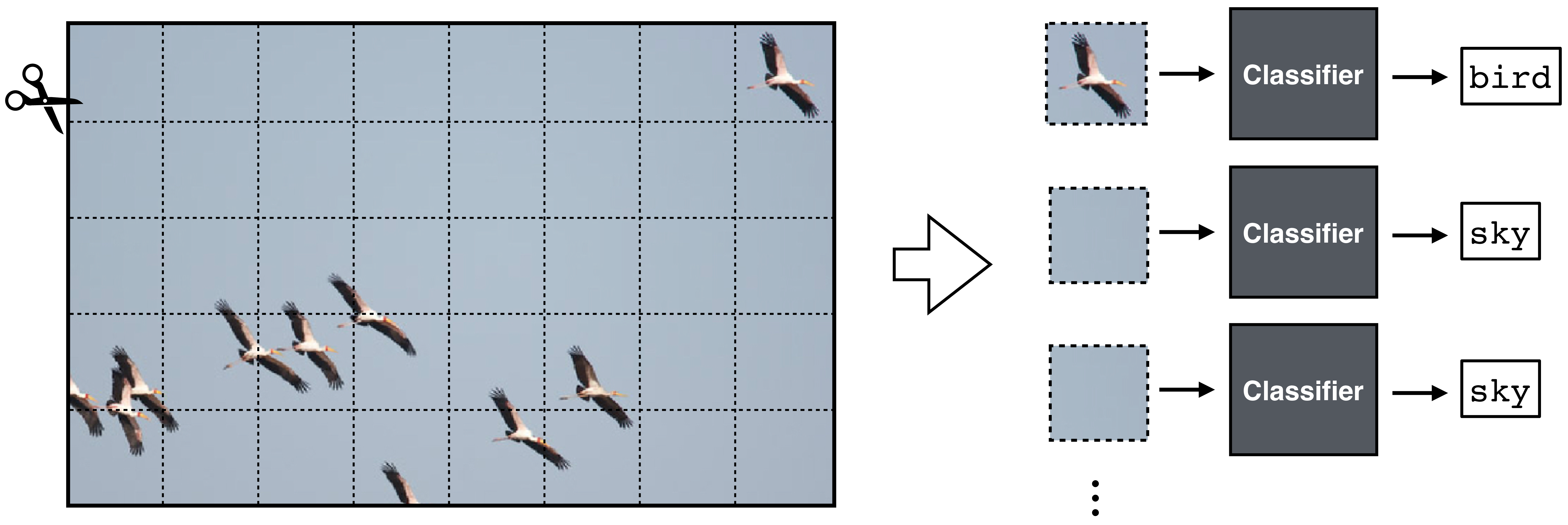
The key idea of CNNs is to chop up the input image into little patches, and then process each patch independently and identically. The gist of this is captured in Figure 24.1:
CNNs are also well suited to processing many other spatial or temporal signals, such as geospatial data or sounds. If there is a natural way to scan across a signal, processing each windowed region separately, then CNNs may be a reasonable choice.
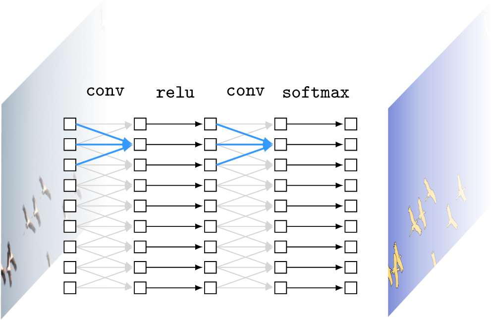
Each patch is processed with a classifier module, which is a neural net. Essentially, this neural net scans across the patches in the input and classifies each. The output is a label for each patch in the input image. If we rearrange these predictions back into the shape of the input image and color code them, we get the below input-output mapping (Figure 24.2):
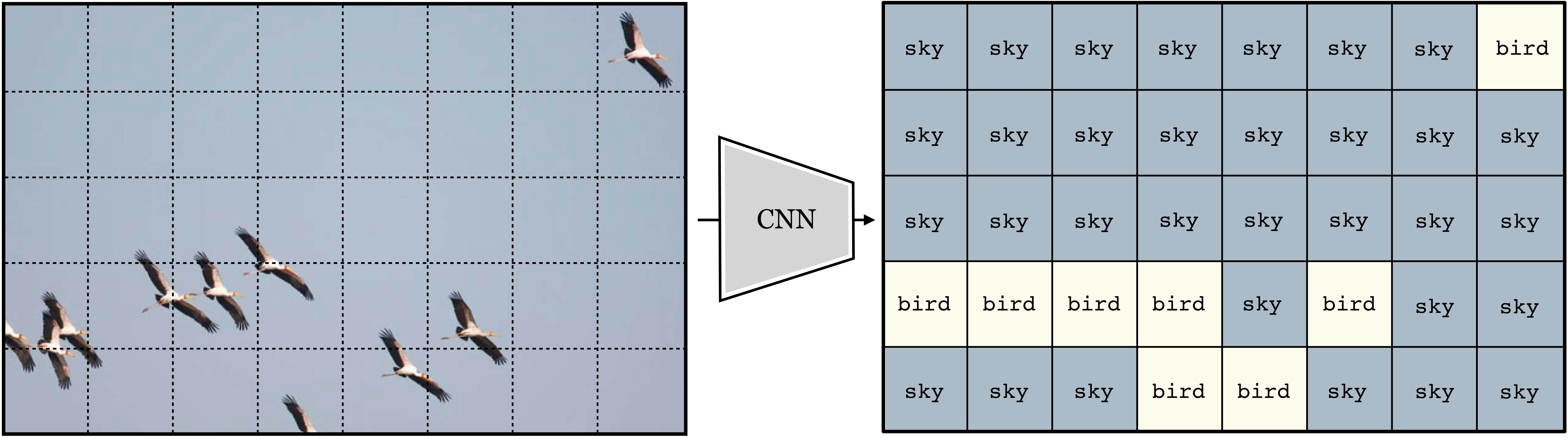
Notice that this is quite different than the neural nets we saw in Chapter 12, which output a single prediction on the entire image; CNNs output a two-dimensional (2D) array of predictions. We may also chop up the image into overlapping patches. If we do this densely, such that each patch is one pixel offset from the last, we get a full resolution image of predictions (Figure 24.3):
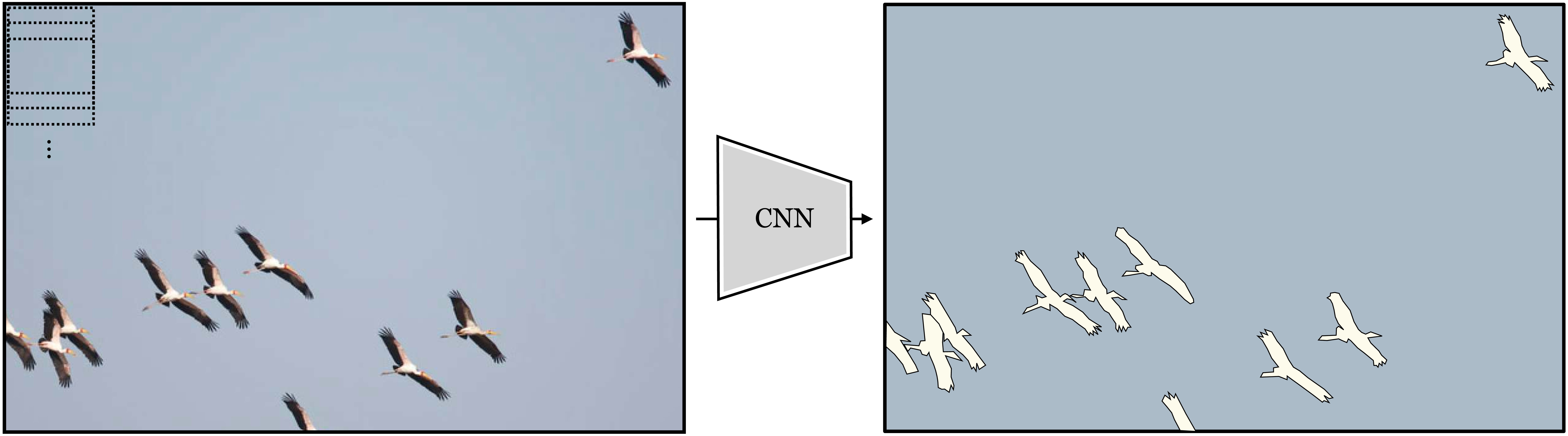
Now that looks impressive! This CNN solved a task known as semantic segmentation, which is the task of assigning a class label to each pixel in an image. One reason CNNs are powerful is because they map an input image to an output image with the same shape, rather than outputting a single label like in the nets we saw in previous chapters. CNNs can also be generalized to input and output other kinds of structures. The key property is that the output matches the topology of the input: an N-dimensional (ND) tensor of inputs will be mapped to an ND tensor of outputs.
Keeping in mind that chopping up and predicting is really all a CNN is doing, we will now dive into the details of how they work.
24.2 Convolutional Layers
CNNs are neural networks that are composed of convolutional layers. A convolutional layer transforms inputs \(\mathbf{x}_{\texttt{in}}\) to outputs \(\mathbf{x}_{\texttt{out}}\) by convolving \(\mathbf{x}_{\texttt{in}}\) with one or more filters \(\mathbf{w}\). A convolutional layer with a single filter looks like this: \[\begin{aligned}\mathbf{x}_{\texttt{out}}= \mathbf{w} \star \mathbf{x}_{\texttt{in}}+ b & \quad\quad \triangleleft \quad \texttt{conv} \end{aligned} \tag{24.1}\] where \(\mathbf{w}\) is the kernel and \(b\) is the bias; \(\theta = [\mathbf{w}, b]\) are the parameters of this layer.
In this chapter, we deviate slightly from our usual notation and use lowercase for convolutional filter \(\mathbf{w}\), regardless of whether the kernel is a 1D array, a 2D array, or an ND array.
Recalling the definition of the operator \(\star\) from Chapter 15, we give here an example of a convolutional layer over a 2D array \(\mathbf{x}_{\texttt{in}}\), using a square kernel of size \(2K+1 \times 2K+1\):
\[\begin{aligned}x_{\texttt{out}}[n,m] = b + \sum_{k_1,k_2=-K}^K w[k_1,k_2] x_{\texttt{in}}[n+k_1,m+k_2] & \quad\quad \\ \triangleleft \quad \texttt{conv}\quad \text{(expanded)} \end{aligned} \tag{24.2}\]
“Convolutional” layers in deep nets are typically actually defined as cross-correlations (\(\star\)) and we stick to that convention in this book. We need not worry about the misnomer because whether you implement the layers with convolution or cross-correlation usually makes no difference for learning. This is because both span an identical hypothesis space (any cross-correlation can be converted to an equivalent convolution by flipping the filter horizontally and vertically).
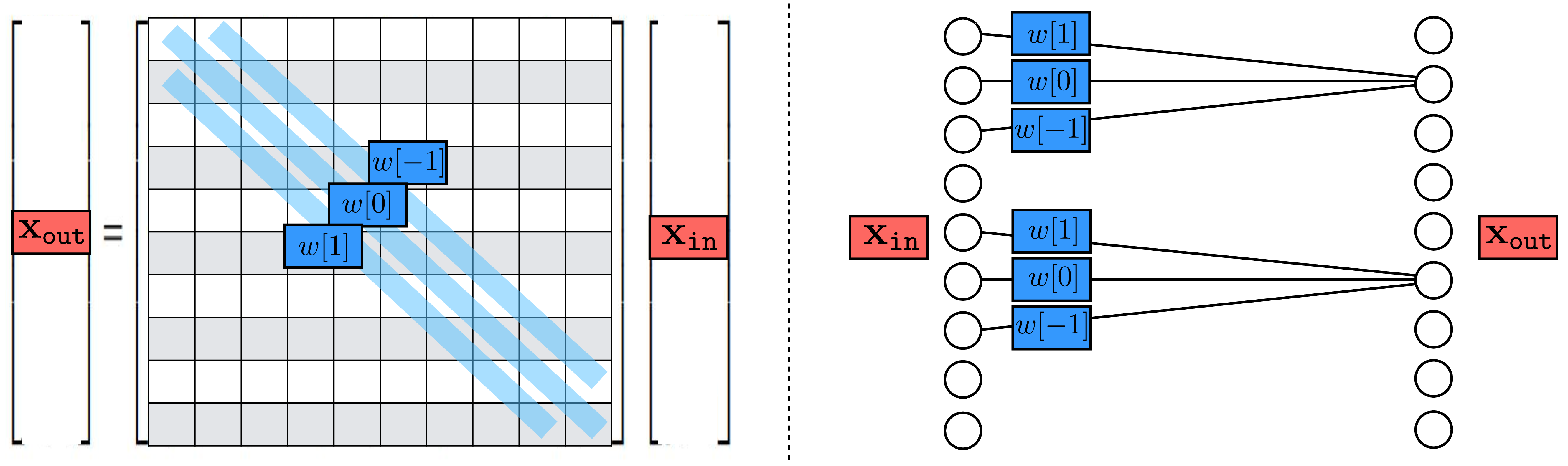
As discussed in Chapter 15, convolution is just a special kind of linear transform. Similarly, a convolutional layer is just a special kind of linear layer. It is a linear layer whose matrix \(\mathbf{W}\) is Toeplitz. We can view it either as a matrix or as a neural net, as shown in Figure 24.4, which shows the case of a one-dimensional (1D) convolution over a 1D signal \(\mathbf{x}_{\texttt{in}}\), with zero bias.
We already saw that convolutional filters are useful for image processing in Foundations of Image Processing and Linear Filters. In those sections, we introduced a variety of hand-designed filter banks with useful properties. A CNN instead learns an effective filter bank.
24.2.1 Multi-Input, Multi-Output Convolutional Layers
In image processing, convolution usually refers to filtering a 1-channel signal and producing a 1-channel output, e.g., filtering a grayscale image and producing a scalar-valued response image. In neural networks, convolutional layers are more general, and typically map a multichannel input to a multichannel output. In this section we define how to handle multichannel inputs, then how to handle multichannel outputs, and then put them together to define the fully general convolutional layer.
Multichannel inputs
Suppose we have an RGB image \(\mathbf{x}_{\texttt{in}}\in \mathbb{R}^{3 \times N \times M}\). To apply a convolutional layer to such a multichannel image we simply use a multichannel filter \(\mathbf{w} \in \mathbb{R}^{C \times K \times K}\), and filter each input channel with the corresponding filter channel, then sum the responses: \[\begin{aligned} \mathbf{x}_{\texttt{out}}= \sum_{c} \mathbf{w}[c,:,:] \star \mathbf{x}_{\texttt{in}}[c,:,:] + b[c] & \quad \triangleleft \quad\texttt{conv}\quad \text{(multichannel in)} \end{aligned}\]
Multichannel outputs
Above we saw a convolutional layer with just a single filter. More commonly each convolutional layer in a neural network will apply a set of filters, i.e. a filter bank. If we have a bank of \(C\) filters \(\mathbf{w}_0, \ldots, \mathbf{w}_{C-1}\), and apply them to a grayscale input image \(\mathbf{x}_{\texttt{in}}\in \mathbb{R}^{N \times M}\), we get \(C\) output images: \[\begin{aligned} \mathbf{x}_{\texttt{out}}[0,:,:] &= \mathbf{w}[0,:,:] \star \mathbf{x}_{\texttt{in}}+ b[0]\\ &\vdots \nonumber\\ \mathbf{x}_{\texttt{out}}[C,:,:] &= \mathbf{w}[C-1,:,:] \star \mathbf{x}_{\texttt{in}}+ b[C-1] \end{aligned} \tag{24.3}\]
Now \(\mathbf{x}_{\texttt{out}}\) is an image with \(C\) channels. Each channel is the response of the input image to one of the filters.
We use the term “image” to refer to any 2D array of measurements or features. An image does not have to be a conventional photograph.
We call each of these channels a feature map, as it shows some features of the input, such as where the vertical edges are.
Multi-Input, Multi-Output
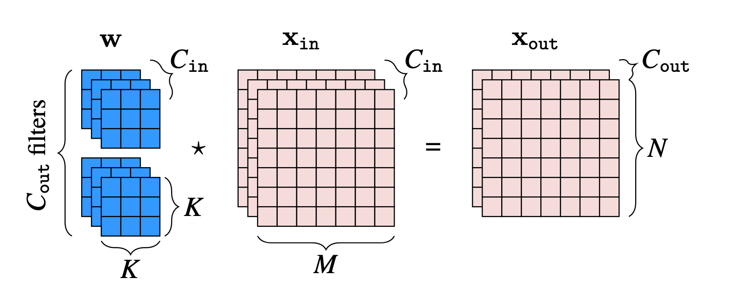
Putting both of the above together, we can define a general convolutional layer that maps a signal with \(C_{\texttt{in}}\) input channels to a signal with \(C_{\texttt{out}}\) output channels. Here is what this looks like for an image \(\mathbf{x}_{\texttt{in}}\in \mathbb{R}^{C_{\texttt{in}}\times N \times M}\), where \(c_2\) indexes the output channel, with \(c_2 \in \{0, \ldots, C_{\texttt{out}}-1\}\):
\[\begin{aligned}\mathbf{x}_{\texttt{out}}[c_{\texttt{2}},:,:] = \sum_{c_{\texttt{1}}=1}^{C_{\texttt{in}}} \mathbf{w}[c_{\texttt{1}},c_{\texttt{2}},:,:] \star \mathbf{x}_{\texttt{in}}[c_{\texttt{1}},:,:] + b[c_{\texttt{2}}] & \quad \triangleleft \quad\texttt{conv}\quad \text{(multi-in-out)} \end{aligned} \tag{24.4}\]
Notation for multichannel convolutions can get hard to keep track of, so let’s spell out a few of the pieces here, which are also visualized in Figure 24.5:
\(\mathbf{x}_{\texttt{in}}[c_{\texttt{1}},:,:]\) is the \(c_{\texttt{1}}\)-th channel of the input signal.
The filter bank is \(C_{\texttt{out}}\) filters, \([\mathbf{w}[:,0,:,:], \ldots, \mathbf{w}[:,C_{\texttt{out}}-1,:,:]]\), each of which applies one convolutional filter per input channel and then sums the responses over all these filters.
This convolutional layer maps inputs \(\mathbf{x}_{\texttt{in}}\in \mathbb{R}^{C_{\texttt{in}}\times N \times M}\) to outputs \(\mathbf{x}_{\texttt{out}}\in \mathbb{R}^{C_{\texttt{out}}\times N \times M}\).
The filter bank is represented by a tensor \(\mathbf{w} \in \mathbb{R}^{C_{\texttt{in}}\times C_{\texttt{out}}\times K \times K}\), where \(K\) is the (spatial, square) kernel size.
It’s important to get comfortable with the shapes of the data and parameter tensors that get processed through different neural architectures. This is essential when designing and building these architectures, and when analyzing and debugging them. Let’s go through an example with concrete numbers. Consider data \(\mathbf{x}_{\texttt{in}}\), which is an RGB image of size \(128 \times 128\) pixels. We will pass it through a convoluational layer that applies a bank of \(3 \times 3\) filters (this refers to the spatial extent of the filters). We omit the bias terms for simplicity. The output ends up being a \(96 \times 128 \times 128\) tensor, as shown in Figure 24.6.
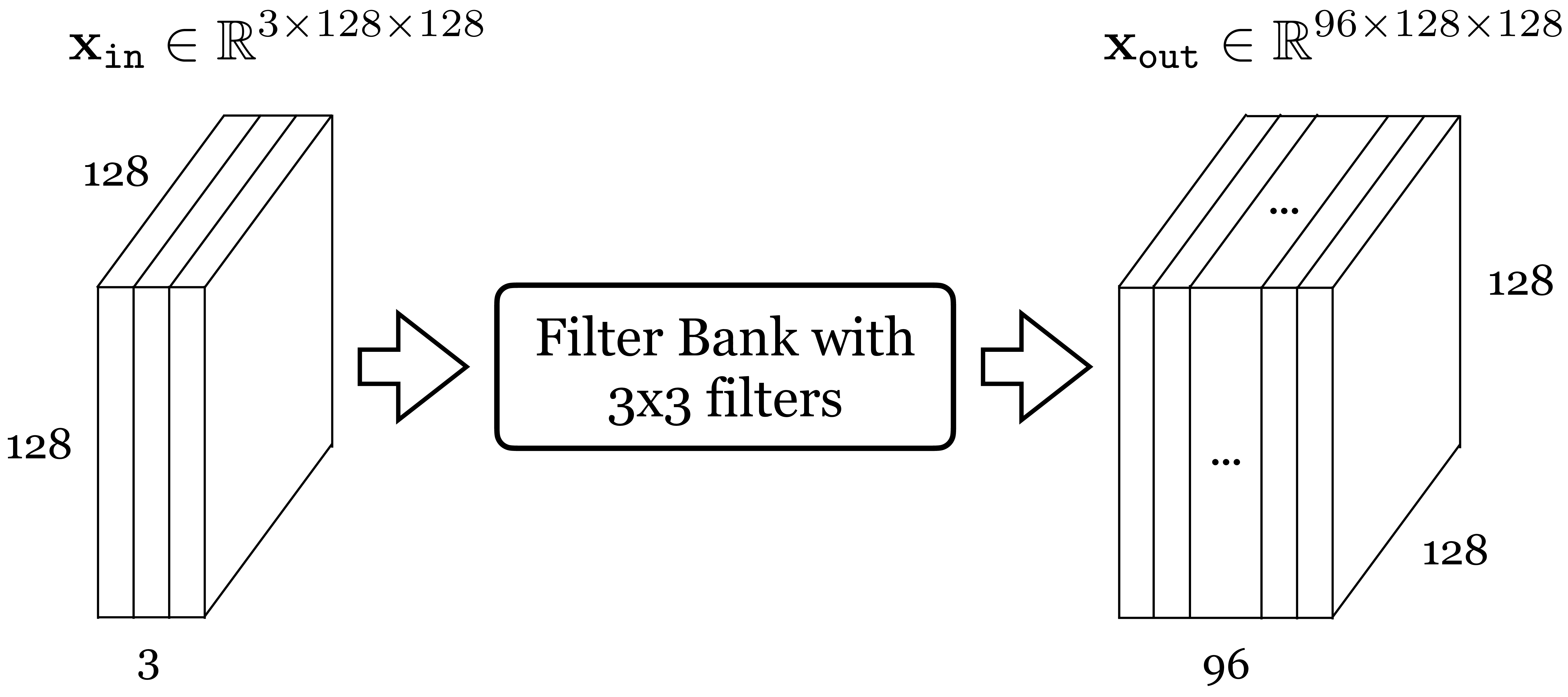
To check your understanding, you should be able to answer the following questions:
How many parameters does each filter have? (A) 9, (B) 27, (C) 96, (D) 864
How many filters are in the filter bank? (A) 3, (B) 27, (C) 96, (D) can’t say
The answers are given in the footnote.1
1 The answers are 1-B, 2-C.
24.2.2 Strided Convolution
Convolutional layers, as defined previously, maintain the spatial resolution of the signal they process. However, commonly it is sufficient, or even desirable, to output a lower resolution. This can be achieved with strided convolution:
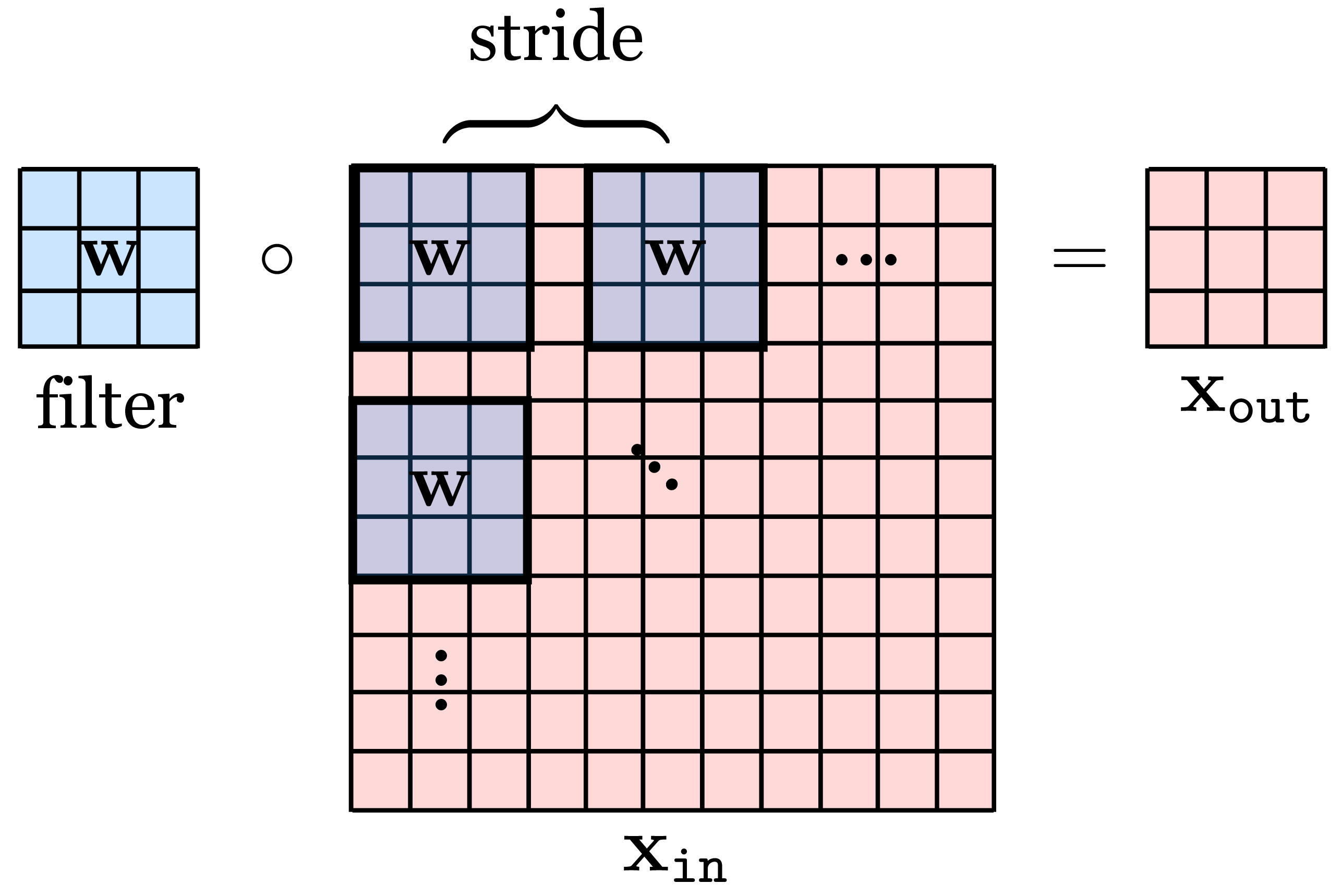
\[\begin{aligned}x_{\texttt{out}}[n,m] = b + \sum_{k_1,k_2=-K}^K w[k_1,k_2] x_{\texttt{in}}[s_n n-k_1,s_m m-k_2] & \quad\quad \triangleleft \quad \texttt{conv}\quad \text{(strided)} \end{aligned} \tag{24.5}\] where \(s_n\) and \(s_m\) are the strides in the vertical and horizontal directions, respectively.
Here and below, we define operations for the simplest case of convolution of a single square filter with a single channel 2D signal. All these operations can be straightforwardly extended for the multichannel in, multichannel out case, and for ND signals, and for non-square kernels. We leave it as an exercise for the reader to write out these variations as needed.
Commonly we use the same stride \(s_n = s_m = s\). A convolution layer with these strides performs a mapping \(\mathbb{R}^{M \times N} \rightarrow \mathbb{R}^{N/s_n \times M/s_m}\). In order to make this mapping well-defined, we require that \(N\) or \(M\) are divisible by \(s_n\) and \(s_m\), respectively; if they are not, we may may pad (or crop) the input until they are.
Strided convolution looks like this (Figure 24.7):
Strided convolutions can significantly reduce the computational cost and memory requirements when a neural network is large. However, strided convolution can decrease the quality of the convolution. Let’s look at one concrete example where the kernel is the 2D Laplacian: \[\mathbf{w} =\begin{bmatrix} 0 ~& -1 ~& 0 \\ -1 ~& 4 ~& -1\\ 0~& -1 ~& 0 \end{bmatrix}\]
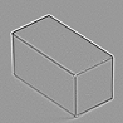
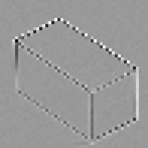
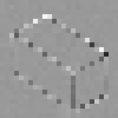
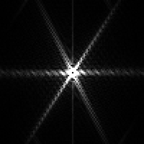
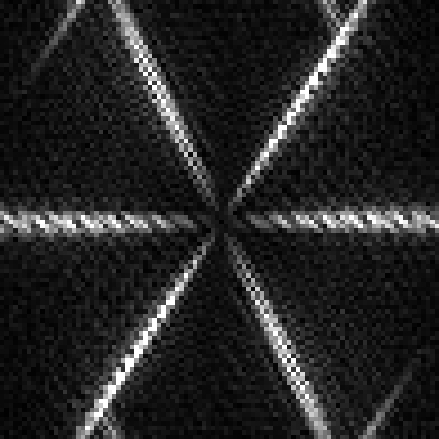
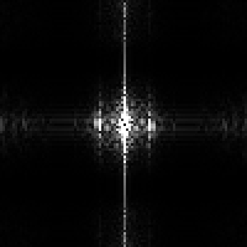
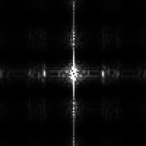
As we saw in Chapter 18, this filter detects boundaries on images. Figure 24.8 shows an input image, and the result of strided convolution with the Laplacian kernel with strides 1, 2, and 4. The second row shows the magnitude of the discrete Fourier transforms (DFT).
| Input | Stride 1 | Stride 2 | Stride 4 |
|---|---|---|---|
 |
 |
 |
 |
 |
 |
 |
 |
The result with stride 1 looks fine, and it is the output we would expect. However, stride 2 starts showing some artifacts on the boundaries, and stride 4 shows very severe artifacts, with some boundaries disappearing. The DFTs make the artifacts more obvious. In the stride 2 result we can see severe aliasing artifacts that introduce new lines in the Fourier domain that are not present in the DFT of the input image.
One can argue that these artifacts might not be important when the kernel is being learned. Indeed, the learning could search for kernels that minimize the artifacts due to aliasing as those probably increase the loss. Also, as each layer is composed of many channels, the set of learned kernels could learn to compensate for the aliasing produced by other channels. However, this reduces the space of useful kernels, and the learning might not succeed in removing all the artifacts.
24.2.3 Dilated Convolution
Dilated convolution is similar to strided convolution but spaces out the filter itself rather than spacing out where the filter is applied to the image: \[\begin{aligned} x_{\texttt{out}}[n,m] = b + \sum_{k_1,k_2=-K}^K w[k_1,k_2] x_{\texttt{in}}[n-d_kk_1,m-d_kk_2] & \quad\quad \triangleleft \quad \texttt{conv}\quad \text{(dilated)} \end{aligned} \tag{24.6}\]
Here we dilate by factor \(d_k\) in both spatial dimensions but we could choose a different dilation in each dimension. Or, we could even dilate in the channel dimension, if we were using a multichannel convolution, but this is uncommon.
An example of a dilated filter is visually shown in Figure 24.9:
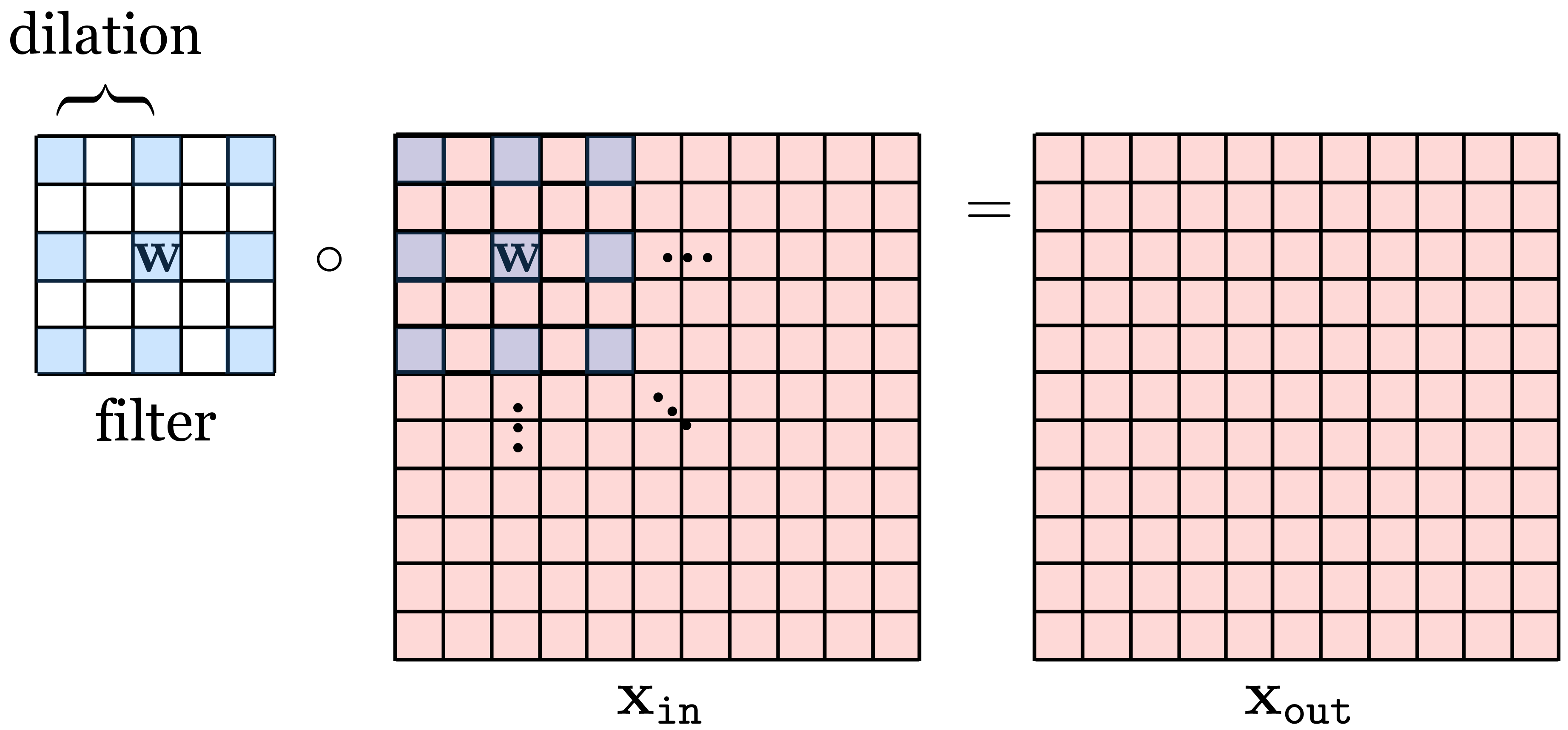
As can be seen in the visualization, dilation is a way to achieve a filter with large kernel while only requiring a small number of weights. The weights are just spaced out so that a few will cover a bigger region of the image.
As was the case with strided convolution, dilation can also introduce artifacts. Let’s look at one example in detail that illustrates the effect of dilation on a filter. Let’s consider the blur kernel, \(b_{2,2}\):
\[\mathbf{w} = \frac{1}{16}\begin{bmatrix} 1 ~& 2 ~& 1 \\ 2 ~& 4 ~& 2\\ 1~& 2 ~& 1 \end{bmatrix}\]
This filter blurs the input image by computing the weighted average of pixel intensities around each pixel location. But, dilation transforms this filter in ways that change the behavior of the filter, which does not behave as a blur filter any longer.
We saw that the 1D signal \([-1, 1, -1, ...]\) convolved with \([1,2,1]\) outputs zero. However, check what happens when we convolve the input with the dilated kernel \([1, 0, 2, 0, 1]\).
The next figure shows the kernel with dilations \(d_k=1\), \(d_k=2\), and \(d_k=4\) together with the magnitude of the DFT of the three resulting kernels (Figure 24.10).
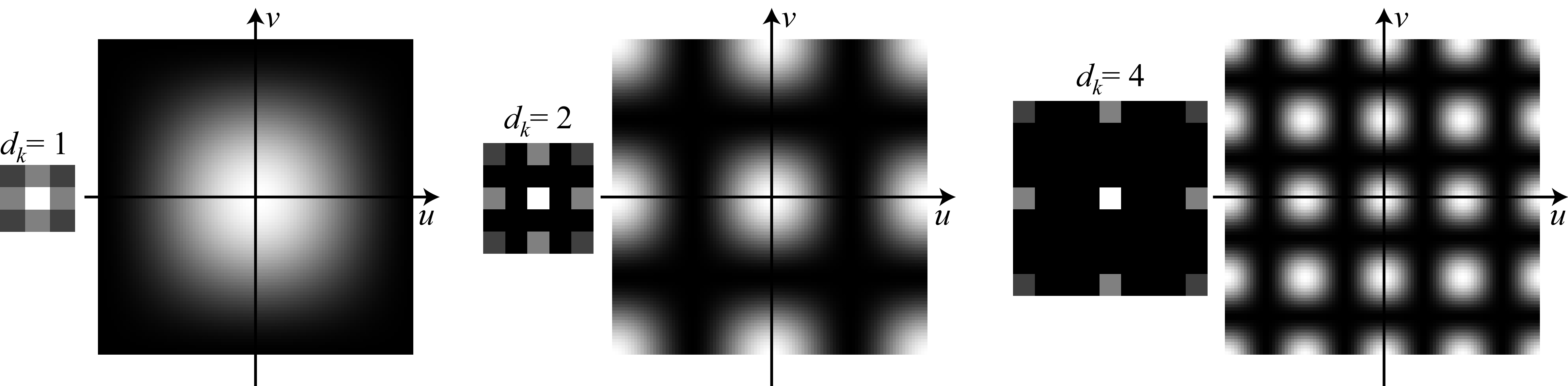
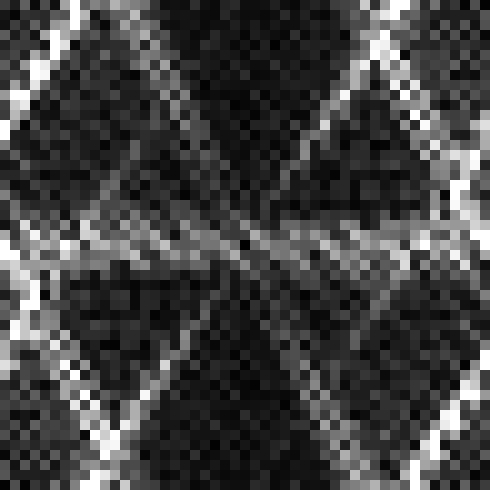
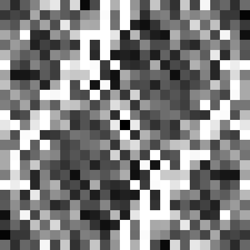
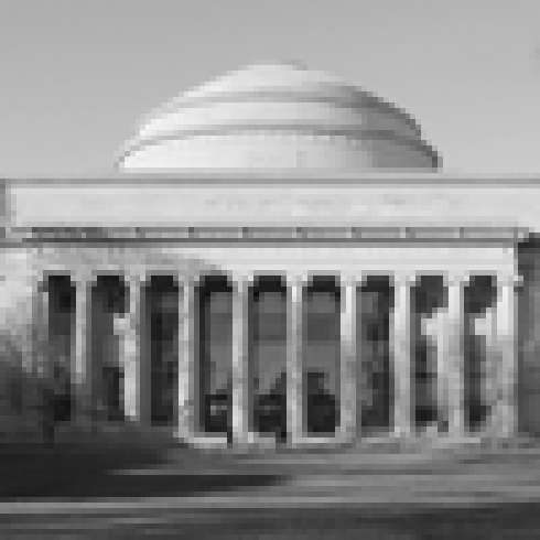
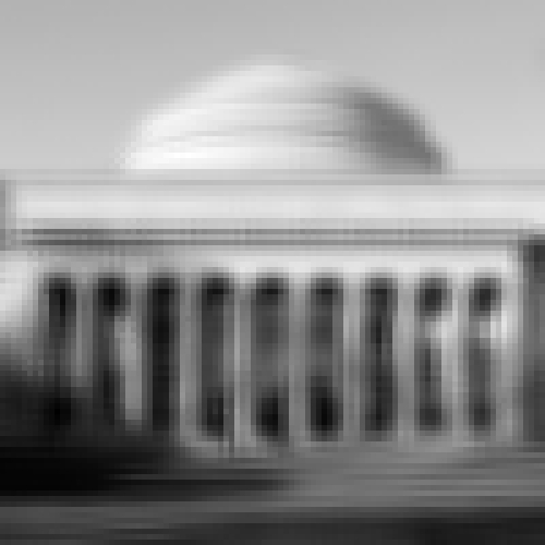
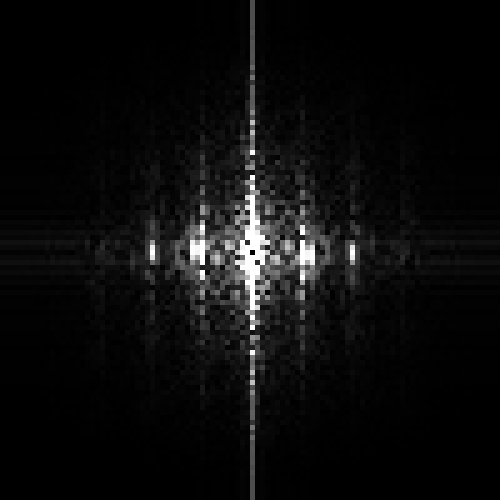
When using the original binomial filter (which corresponds to \(d_k=1\)) the DFT shows that the filter is a low-pass filter. When applying dilation (\(d_k=2\)) the DFT changes and it is not unimodal anymore. It has now eight additional local maximum in high spatial frequencies. With \(d_k=4\), the DFT reveals an even more complex frequency behavior. Figure 24.11 shows one input image and the result of the dilated convolutions with the blur kernel, \(b_{2,2}\), with dilations \(d_k=1\), \(d_k=2\), and \(d_k=4\).
When using the original binomial filter (which corresponds to \(d_k=1\)) the DFT shows that the filter is a low-pass filter. When applying dilation (\(d_k=2\)) the DFT changes and it is not unimodal anymore. It has now eight additional local maximum in high spatial frequencies. With \(d_k=4\), the DFT reveals an even more complex frequency behavior. Figure 24.11 shows one input image and the result of the dilated convolutions with the blur kernel, \(b_{2,2}\), with dilations \(d_k=1\), \(d_k=2\), and \(d_k=4\).
| Input | \(d_k\) = 1 | \(d_k\) = 2 | \(d_k\) = 4 |
|---|---|---|---|
 |
 |
 |
 |
 |
 |
 |
 |
In summary, using dilation increases the size of the convolution kernels without increasing the computations (which is the original desired property) but it reduces the space of useful kernels (which is an undesired property).
There are ways in which dilation can be used to increase the family of useful filters. For instance, by composing three convolutions with \(d_k=1\), \(d_k=2\), and \(d_k=4\) together (Figure 24.12), one can create a kernel that can switch during learning between high and low spatial frequencies and small and large kernels.
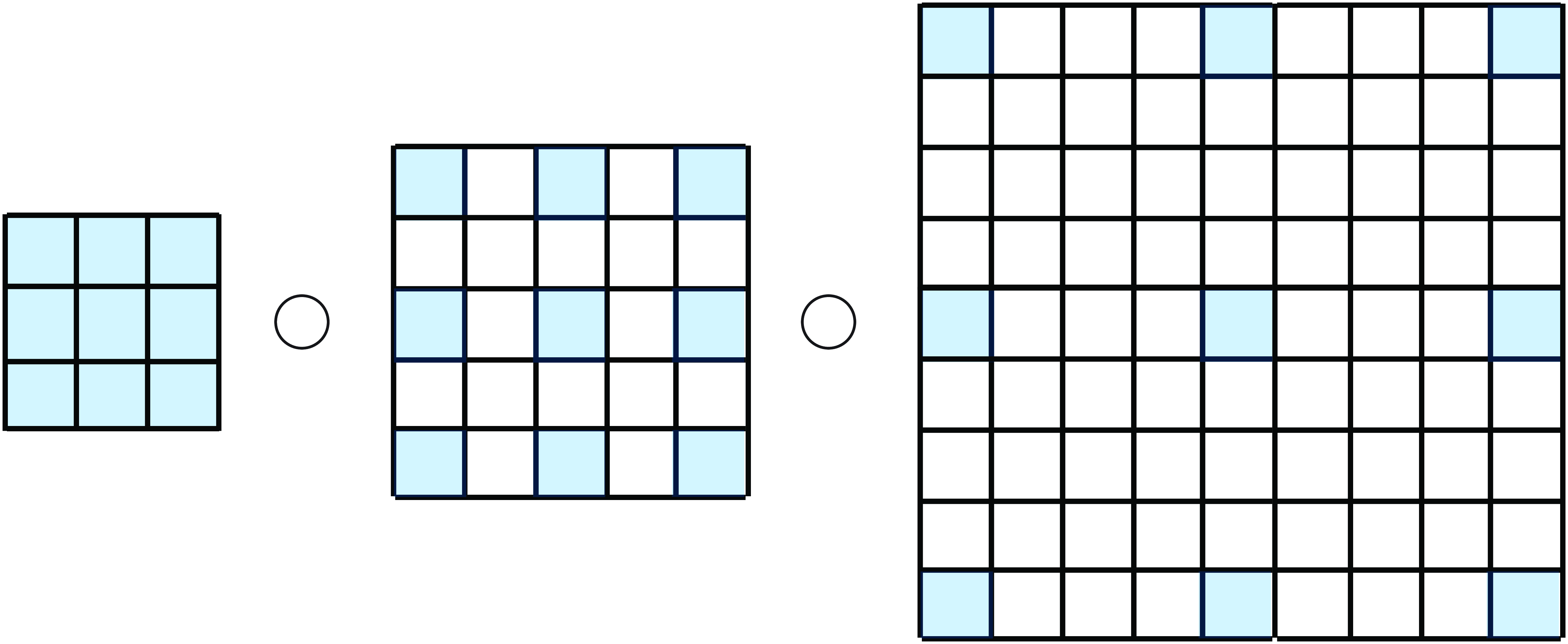
This results in a kernel with a size of \(9 \times 9\) (81 values) defined by 27 values. The relative computational efficiency increases when we cascade more filters with higher levels of dilation. Figure 24.13 shows several multiscale kernels that can be obtained by the convolutions of three dilated kernels. Can you guess which kernels were used?
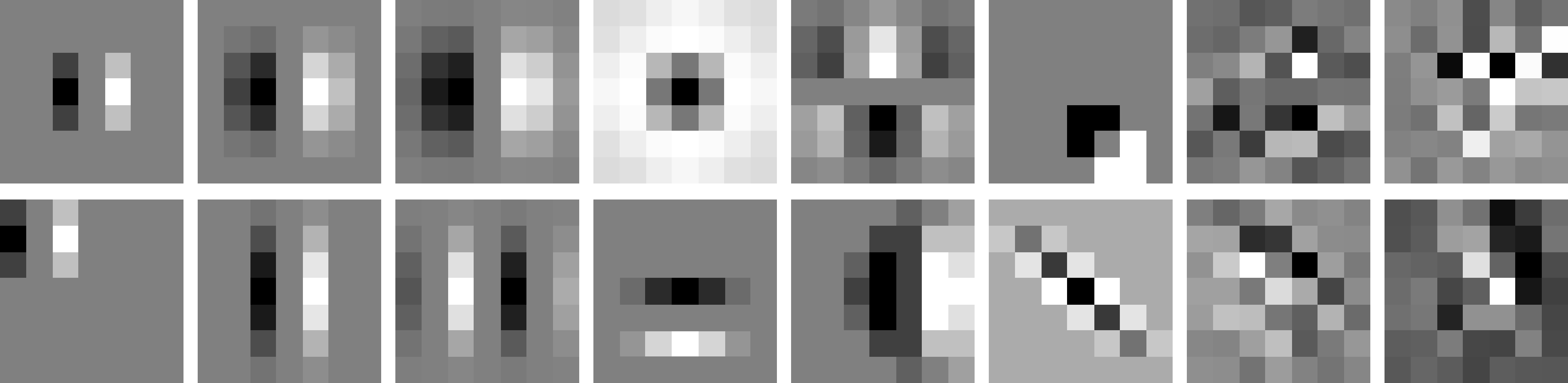
As the figure shows, the cascade of three dilated convolutions can generate a large family of filters with different scales, orientations, shifts, and also other patterns such as corner detectors, long edge detectors, and curved edge detectors. The last four kernels shows the result of convolving three random kernels, which provides further illustration of the diversity of kernels one can build. Each kernel is a \(3 \times 3\) array sampled from a Gaussian distribution.
24.2.4 Low-Rank Filters
Dilation is one way to create a big filter that is parameterized by just a small number of weights, that is, a low-rank filter. This trick can be useful in many contexts where we know that good filters have low-rank structure. Dilation uses this trick to make big kernels, which can capture long-range dependences.
Separable filters are another kind of low-rank filter that is useful in many applications (see Chapter 16). We can create a convolutional layer with separable filters by simply stacking two convolutional layers in sequence, with no other layers in between. The first layer is a filter bank with \(K \times 1\) kernels and the second uses \(1 \times K\) kernels. The composition of these layers is equivalent to a single convolutional layer with \(K \times K\) separable filters. Two examples of such separable filters are given below Figure 24.14):
When convolving one row and one column vector, \(\mathbf{w} = \mathbf{u}^\mathsf{T} \circ \mathbf{v}\), the result is the outer product: \(w \left[n,m \right] = u\left[n \right] v\left[m \right]\).

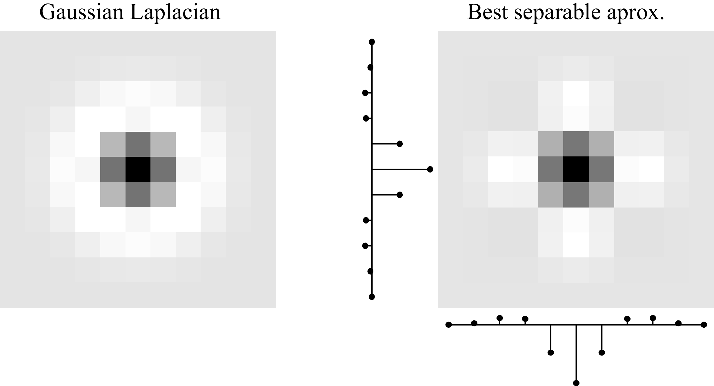
Some important kernels are nonseparable but can be approximated by a linear combination of a small number of separable filters. For instance, the Gaussian Laplacian is nonseparable but can be approximated by a separable filter as shown here (Figure 24.15):
The diagonal Gaussian derivative is another nonseparable kernel. When using a \(3 \times 3\) kernel to approximate it we have:
\[\mathbf{w} = \begin{bmatrix} 0 ~& -2 ~& -2 \\ 2 ~& 0 ~& -2\\ 2~& 2 ~& 0 \end{bmatrix}\]
But we know from Chapter 18 that this kernel can be written as a linear combination of two separable kernels: \(\mathbf{w} = \text{Sobel}_x + \text{Sobel}_y\), as defined in equation (Equation 18.3). In general, any \(M \times N\) filter can be decomposed as a linear sum of \(\min(N,M)\) separable filters. The separable filters can be obtained by applying the singular value decomposition (SVD) to the kernel array \(\mathbf{w}\). The SVD results in three matrices, \(\mathbf{U}\), \(\mathbf{S}\) and \(\mathbf{V}\), so that \(\mathbf{w} = \mathbf{U} \mathbf{S} \mathbf{V}^\mathsf{T}\), where the columns of \(\mathbf{U}\) and \(\mathbf{V}\) are the separable 1D filters and the diagonal values of the diagonal matrix \(\mathbf{S}\) are the linear weights. Computational benefits are only obtained when using small linear combinations for large kernels. Also, in a neural network, one could use only separable filters for all the units and the learning could discover ways of combining them in order to build more complex, nonseparable kernels.
24.2.5 Downsampling and Upsampling Layers
In Chapter 23 we saw image pyramids and showed how they can be used for analysis and synthesis. CNNs can also be structured as analysis and synthesis pyramids, and this is a very powerful tool. To create a pyramid we just need to introduce a way of downsampling the signal during analysis and upsampling during synthesis. In CNNs this is done with downsampling and upsampling layers.
Downsampling layers transform the input tensor to an output tensor that is smaller in the spatial dimensions: \(\mathbb{R}^{N \times M} \rightarrow \mathbb{R}^{N/s_n \times M/s_m}\). We already saw one kind of downsampling layer, strided convolution, which is equivalent to convolution followed by subsampling. Another common kind of downsampling layer is pooling, which we will encounter in Section 24.3.1.
Upsampling layers perform the opposite transformation, outputting a tensor that is larger in the spatial dimensions than the input: \(\mathbb{R}^{N \times M} \rightarrow \mathbb{R}^{Ns_n \times Ms_m}\).
One kind of upsampling layer can be made as the analogue of strided convolution. Strided convolution convolves then subsamples; this upsampling layer instead dilates the signal then convolves. Starting with a blank image of zeros, \(\mathbf{h} = \mathbf{0}\), we set: \[\begin{aligned} h[ns_n, ms_m] &= x_{\texttt{in}}[n, m] & \quad\quad \triangleleft \quad \texttt{dilation}\\ \mathbf{x}_{\texttt{out}}&= \mathbf{w} \star \mathbf{h} + b & \quad\quad \triangleleft \quad \texttt{conv} \end{aligned} \tag{24.7}\]
This equation applies for all integer values of \(n \in \{1,\ldots,N\}\) and \(m \in \{1,\ldots,M\}\).
Sometimes the combination of these two layers is called an UpConv layer or a deconvolution layer (but note that deconvolution has a different meaning in signal processing).
24.3 Nonlinear Filtering Layers
All the operations we have covered above are linear (or affine). It is also possible to define filters that are nonlinear. Like convolutional filters, these filters slide across the input tensor and process each window identically and independently, but the operation they perform is a nonlinear function of the local window.
24.3.1 Pooling Layers
Pooling layers are downsampling layers that summarize the information in a patch using some aggregate statistic, such as the patch’s mean value, called mean pooling, or its max value, called max pooling, defined as follows:
\[\begin{aligned} x_{\texttt{out}}[i]= \max_{i \in \mathcal{N}(i)} x_{\texttt{in}}[i]& \quad\quad \triangleleft \quad \texttt{max pooling}\\ x_{\texttt{out}}[i]= \frac{1}{|\mathcal{N}|} \sum_{i \in \mathcal{N}(i)} x_{\texttt{in}}[i]& \quad\quad \triangleleft \quad \texttt{mean pooling} \end{aligned} \tag{24.8}\]
The \(\mathcal{N}(i)\) indicates the set of indices in the same patch as index \(i\).
Like all downsampling layers, pooling layers can be used to reduce the resolution of the input tensor, removing high-frequency information in the signal. Pooling is also particularly useful as a way to achieve invariance. Convolutional layers produce outputs that are equivariant to translations of their input. Pooling is a way to convert equivariance into invariance. For example, suppose we have run a convolutional filter that detects vertical edges. The output is a response map that is large wherever there was a vertical edge in the input image. Now if we run a max pooling filter across this response map, it will coarsen the map, resulting in a large response anywhere near where there was a vertical edge in the input image. If we use a max pooling filter with large enough neighborhood \(\mathcal{N}\), the output will be invariant to the location of the edge in the input image.
Pooling can also be performed across channels, and this can be a way to achieve additional kinds of invariance. For example, suppose we have a convolutional layer that applies a filter bank of oriented edge detector filters, where each filter looks for edges at a different orientation. Now if we max pool across the channels output by this filter bank, the resulting feature map will be large wherever an edge of any orientation was found. Normally, we are not looking for edges but for more complicated patterns, but the same logic applies. First run a bank of filters that look for the pattern at \(k\) different orientations. Then pool across these \(k\) channels to detect the pattern regardless of its orientation. This can be a great way for a CNN to recognize objects even if they appear with various rotations within the image. Of course we usually do not hand-define this strategy but it is one the CNN can learn to use if given channelwise pooling layers.
24.3.2 Global Pooling Layers
One extreme of pooling is to pool over the entire spatial extent of the feature map. Global pooling is a function that maps a \(C \times M \times N\) tensor into a vector of length \(C\), where \(C\) is the number of channels in the input.
Global pooling is generally used in layers very close to the output. As before, global pooling can be global average pooling, averaging over all the responses of the feature map, or global max pooling, taking the max of the feature map.
Global pooling removes spatial information from each channel. However, spatial information about input features might be still be available within the output vector if different channels learn to be sensitive to features at different spatial positions.
24.3.3 Local Normalization Layers
Another kind of nonlinear filter is the local normalization layer. These layers normalize each activation in a feature map by statistics the adjacent activations within some neighborhood. There are many different choices for the type of normalization (\(L_1\) norm, \(L_2\) norm, standardization, etc.) and many different choices for the shape of the neighborhood, such as a square patch in the spatial dimensions, a set of channels, and so on. Each of these choices leads to different kinds of normalization filters with different names. One that is historically important but no longer frequently used is the local response normalization, or LRN, filter that was introduced in the AlexNet paper [1]. This filter has the following form: \[\begin{aligned} x_{\texttt{out}}[c,n,m] = x_{\texttt{in}}[c,n,m] / \left( \gamma + \alpha \sum_{i=\max(1,c-l)}^{\max(C,c+l)} x_{\texttt{in}}[i,n,m]^2 \right) ^\beta \quad\quad \triangleleft \quad\texttt{LRN} \end{aligned} \tag{24.9}\] where \(\alpha\), \(\beta\), \(\gamma\), and \(l\) are hyperparameters of the layer. This layer normalizes each activation by the sum of squares of the activations in a window of adjacent channels.
Although local normalization is a common structure within the brain, it is not very frequently used in current neural networks, which more often use global normalization layers like batchnorm or layernorm (which we saw in Chapter 12.
24.4 A Simple CNN Classifier
CNNs are deep nets that stack convolutional layers in a series, interleaved with nonlinearities. CNNs also frequently use downsampling and upsampling layers, pooling layers, and normalization layers, as described above.
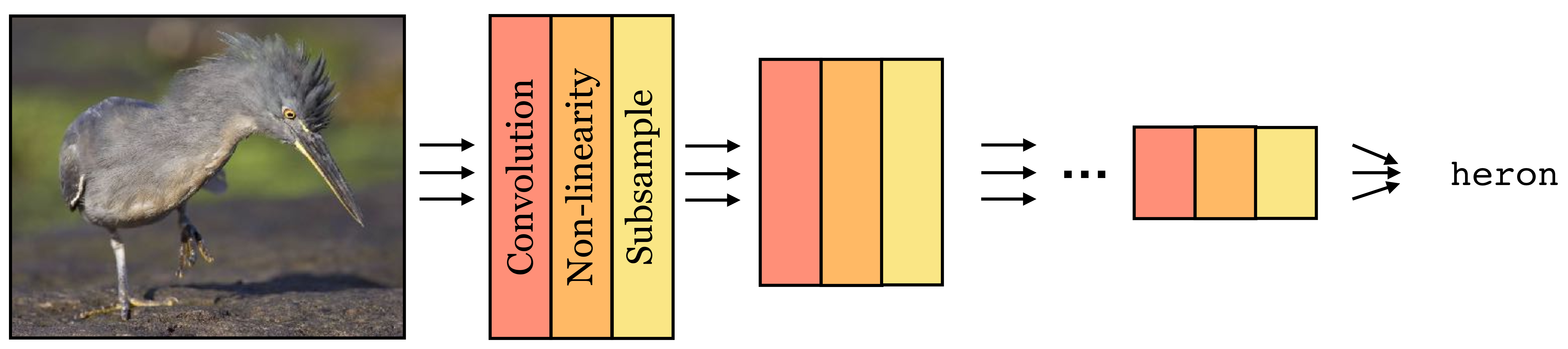
CNNs come in a large variety of architectures, each suited to a different kind of problem. We will see some of these architectures in Section 24.11. For now we will focus on just one simple architecture that is suited to image classification. This architecture progressively downsamples the image until the last layer makes a single global prediction of the image label (Figure 24.16):
We will now walk through an example of such a classifier. Let \(\mathbf{x} \in \mathbb{R}^{M \times N}\) be a black and white image. To process this image, we could use a simple CNN with two convolutional layers, defined as follows:
\[\begin{align} \mathbf{z}_1[c,:,:] &= \mathbf{w}[c,:,:] \star \mathbf{x} + b[c] &\triangleleft \quad \texttt{conv}: [M \times N] \rightarrow [C \times M \times N]\\ h[c,n,m] &= \max(z_1[c,n,m],0) &\triangleleft \quad \texttt{relu}: [C \times M \times N] \rightarrow [C \times M \times N]\\ z_2[c] &= \frac{1}{NM} \sum_{n,m} h[c,n,m] &\triangleleft \quad \texttt{gap}: [C \times M \times N] \rightarrow [C]\\ \mathbf{z}_{3} &= \mathbf{W} \mathbf{z}_{2} + \mathbf{c} &\triangleleft \quad \texttt{fc}: [C] \rightarrow [K]\\ y[k] &= \frac{e^{-\tau z_3[k]}}{\sum_{l=1}^K e^{-\tau z_3[l]}} &\triangleleft \quad \texttt{softmax}: [K] \rightarrow [K] \end{align}\]
Note that these equations apply for all \(c \in \{0,\ldots,C-1\}\), \(n \in \{0,\ldots,N-1\}\) and \(m \in \{0,\ldots,M-1\}\).
This network has one convolutional layer with \(C\) channels followed by a relu layer. The next layer performs spatial global average pooling (gap), and each channel gets projected into a single number that contains the sum of the outputs of the relu. This results in a representation given by a vector of length \(C\). This vector is then processed by a fully connected layer (fc). A fully connected layer is simply another name for a linear layer that is full rank, that is, every output neuron is connected to every input neuron, and the mapping is described by a \(K \times C\) matrix (plus a bias).
This neural net could be used to solve a \(K\)-way image classification problem (because the output is a \(K\)-way softmax for each input image). We could train it using gradient descent to find the parameters \(\theta = [\mathbf{w}_1, \ldots, \mathbf{w}_C, \mathbf{b}_1, \ldots, \mathbf{b}_C, \mathbf{W}, \mathbf{c}]\) that optimize a cross-entropy loss over training data.
Such a network is also very easy to define in code, once we have a library of primitives for basic operations like convolution and softmax:
# first define parameterized layers
conv1 = nn.conv(channels_in=1, channels_out=C, kernel=k, stride=1)
fc1 = nn.fc(dim_in=C, dim_out=K)

# then run data through network
z1 = conv1(x)
h = nn.relu(z1)
z2 = nn.AvgPool2d(h)
z3 = fc1(z2)
y = nn.softmax(z3)
24.5 A Worked Example
In this section, we will analyze the simple network described in Section 24.4, trained to discriminate between horizontal and vertical lines. Each subsection will tackle one aspect of the analysis that should be part of training any large system: (1) training and evaluation, (2) visualize and understand the network, (3) out-of-domain generalization, and (4) identifying vulnerabilities.
24.5.1 Training and Evaluation
Let’s study one simple classification task. We design a simple image dataset that contains images with lines. The lines can be horizontal or vertical. Each image will contain only one type of line.
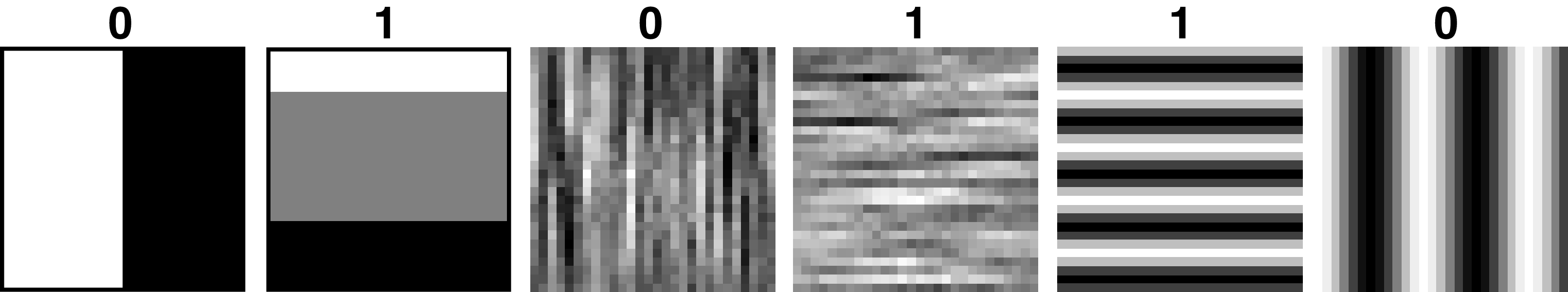
We want to design a CNN that will classify the image according to the orientation of the lines that it contains. We define the two output classes as: \(0\) (vertical) and \(1\) (horizontal). A few samples from the training set are shown in Figure 24.17.
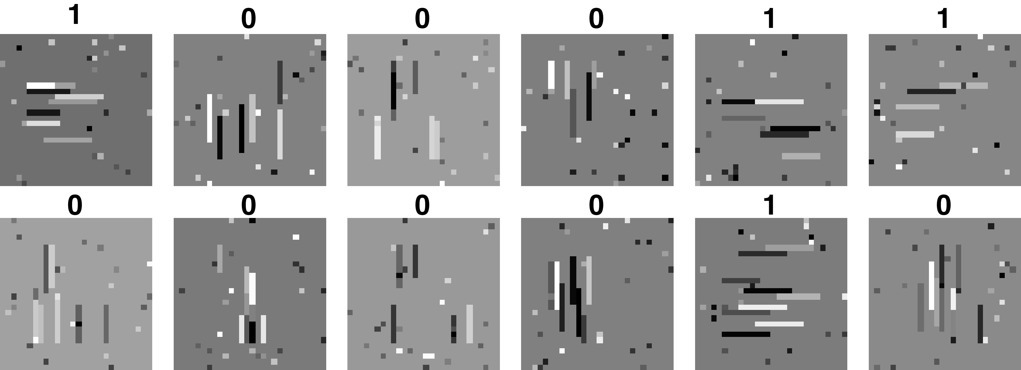
To solve this problem we use the CNN defined before with two convolutional channels \(C=2\) in the first layer. Once we train the network, we can see that it has solve the task perfectly and that the output on the test set is 100 percent correct (there are only three errors out of 10,000 test images). Example images from the test set are shown in Figure 24.18.
24.5.2 Network Visualization
What has the network learned? How is it solving the problem? One important part of developing a system is to have tools to prove, understand, and debug it.
To understand the network it is useful to visualize the kernels. Figure 24.19 shows the two learned \(9 \times 9\) kernels. The first one looks like an horizontal derivative of a Gaussian filter (as we saw in Chapter 18 and the second one looks like a vertical derivative of a Gaussian (maybe closer to a second derivative). In fact, the DFT of each kernel shows that they are quite selective to a particular band on frequency content in the image.

The fully connected layer has learnt the weights: \[\mathbf{W} = \left[ \begin{array}{cc} 2.83 & -2.36 \\ -0.60 & 1.14 \end{array} \right]\] This corresponds to two channel oppositions: the first feature is the vertical output minus the horizontal output, and the second feature computes the horizontal output minus the vertical one.
24.5.3 Out-of-Domain Generalization
What do we learn by analyzing how the trained network works? One interesting outcome is that can we predict how the network we defined before generalizes beyond the distribution of the training set, to out-of-domain test samples.
Another term for out-of-domain is out-of-distribution.
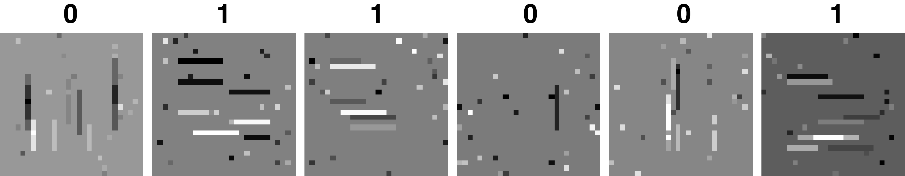
For instance, it seems natural to think that the network should still perform well in classifying whether the image contains vertical or horizontal structures even if they are not lines. We can test this hypothesis by generating images that match our idea of orientation. The following test images (Figure 24.20) contain different oriented structures but no lines, and still captures our notion of what should be the correct generalization of the behavior.
In fact, the network seems to perform correctly even with these new images that come from a distribution different from the training set.
24.5.4 Identifying Vulnerabilities
Does the network solve the task that we had in mind? Can we predict which inputs will make the output fail? Can we produce test examples that to us look right but for which the network produces the wrong classification output? The goal of this analysis is to identify weaknesses in the learned representation and in our training set (missing training examples, biases in our data, limitations of the architecture, etc.).
We saw that the output of the first layer does not really look for lines, instead it looks at where the energy is in the Fourier domain. So, we could fool the classifier by creating lines that for us look like vertical lines, but that have the energy content in the wrong side of the Fourier domain. We saw one trick to do this in Chapter 16: modulation. If we multiply an image containing horizontal lines, by a sinusoidal wave, \(\cos (\pi n / 3)\), we can move the spectral content horizontally as shown in Figure 24.21.
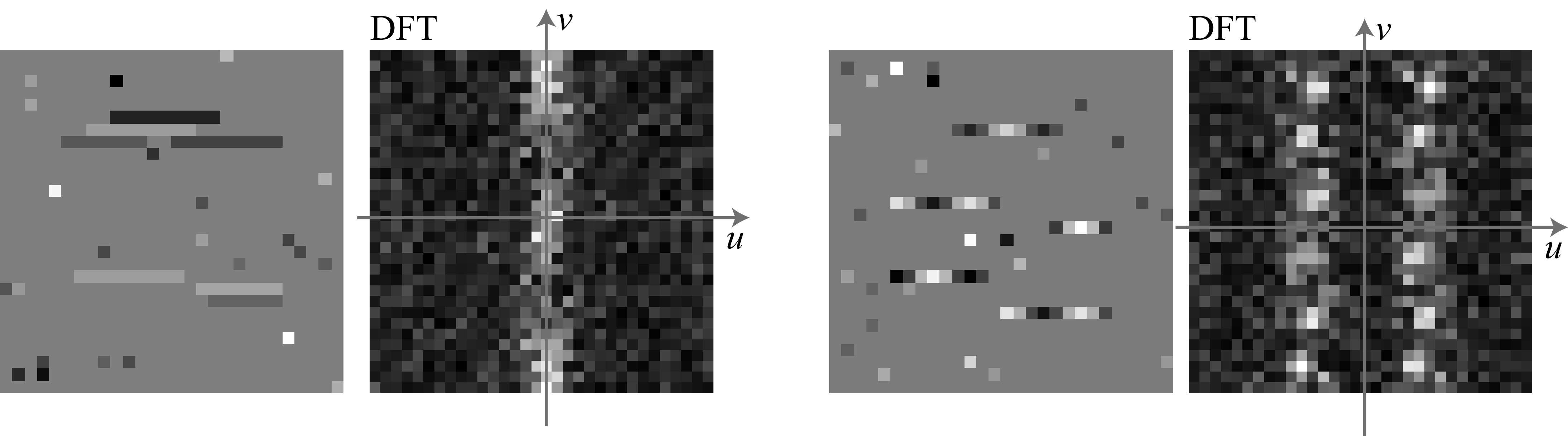
The lines still look horizontal to us, but their spectral content now is higher in the region that overlaps with the vertical line detector learned by the network. Indeed, when the network processes images that have lines with this sinusoidal texture, it produces the wrong classification results for all the images (Figure 24.22)!

We have just designed an adversarial example manually! The question then could be as follows: If it is not detecting line orientations, what is it really detecting? Our analysis of the learned kernels had the answer.
For complex architectures, adversarial examples are obtained as an optimization problem: What is the minimal perturbation of an input that will produce the wrong output in the network?
One way of avoiding this would be to introduce these types of images in the training set and to repeat the whole process.
24.6 Feature Maps in CNNs
One of the most important concepts when working with CNNs is the feature map. A feature map can be a channel of the output of a conv layer (as we defined above) or it can refer to the entire stack of channels at some layer of a network. The idea is that these are features of the input data and the features are arranged in a map – an array that matches the shape of the input data. For images, feature maps are 2D spatial arrays, for videos they are 3D space-time arrays, and so forth.
Figure 24.23 shows the interplay between feature maps and filter banks in a CNN:
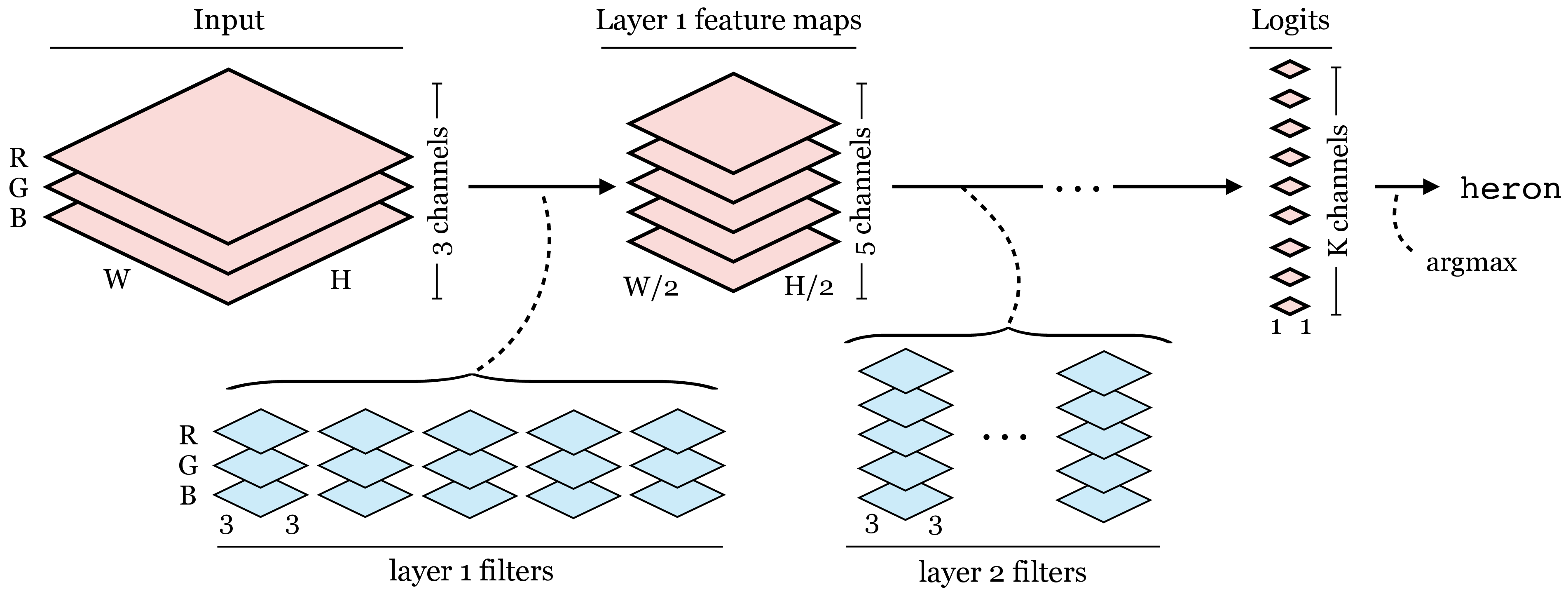
The input to the network is an image and the output is a vector of logits. We can actually think of these inputs and outputs as feature maps as well: the input is just a feature map with red, green, and blue channels and the output is a 1x1 resolution feature map with class logits as the channels.
Now let’s look at the feature maps in a real network, AlexNet [1]. Figure 24.24 shows what these look like after the first and second convolutional layer of the network:
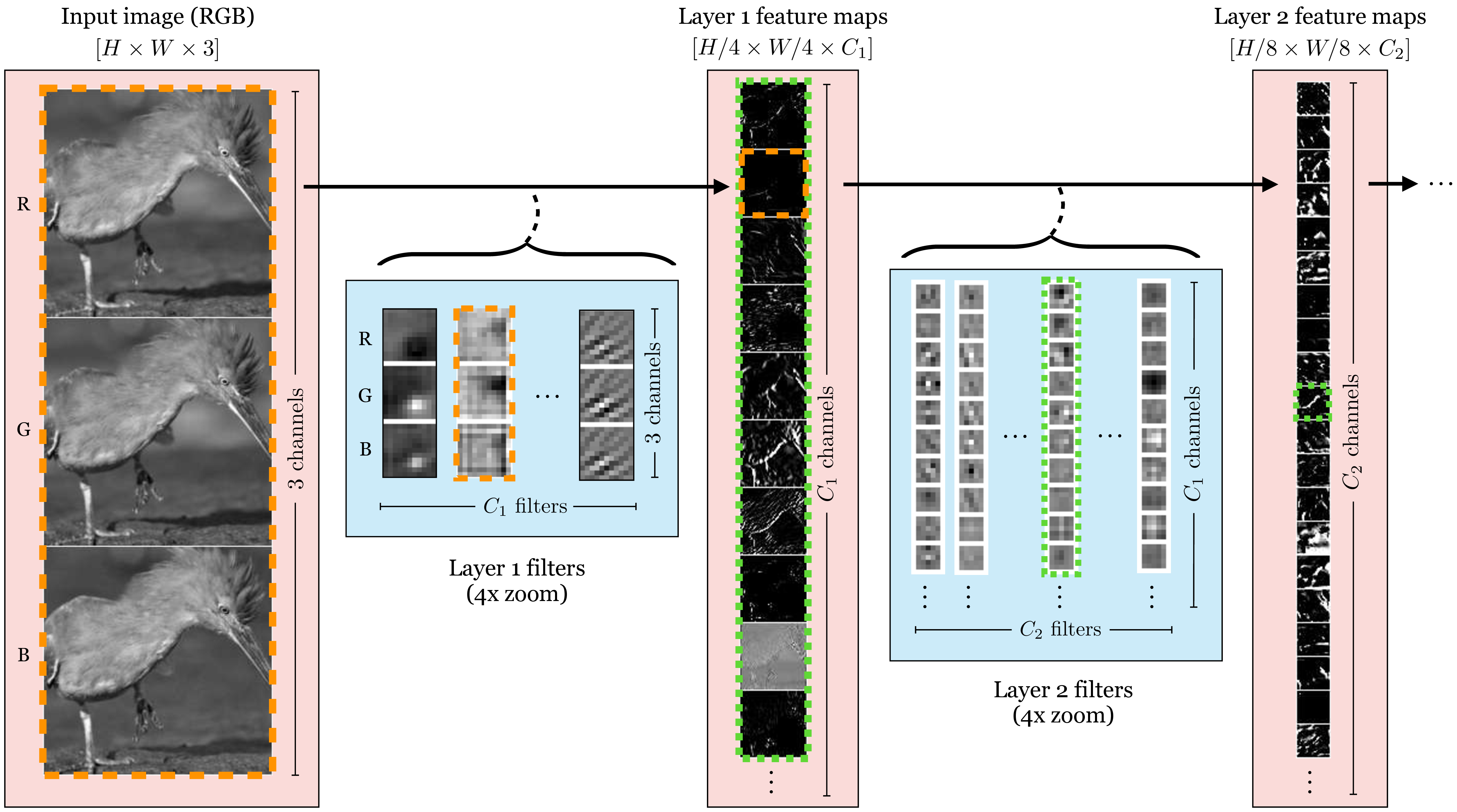
There are a few things to notice in this figure. First, the spatial resolution of the feature maps get lower as we go deeper into the network, and the number of channels increases. This is common in CNNs: each layer downsamples and adds channels to partially compensate for the reduction in resolution. Second, while on the first layer the feature maps are sensitive to basic patterns in the input image – edges, lines, etc – the maps become more abstracted as we go deeper. This is typical of image classifier networks: channels in the shallow layers capture basic image features and channels in the deeper layers increasingly correspond to class semantics (e.g., one channel might be a heatmap of where the “bird” pixels are).
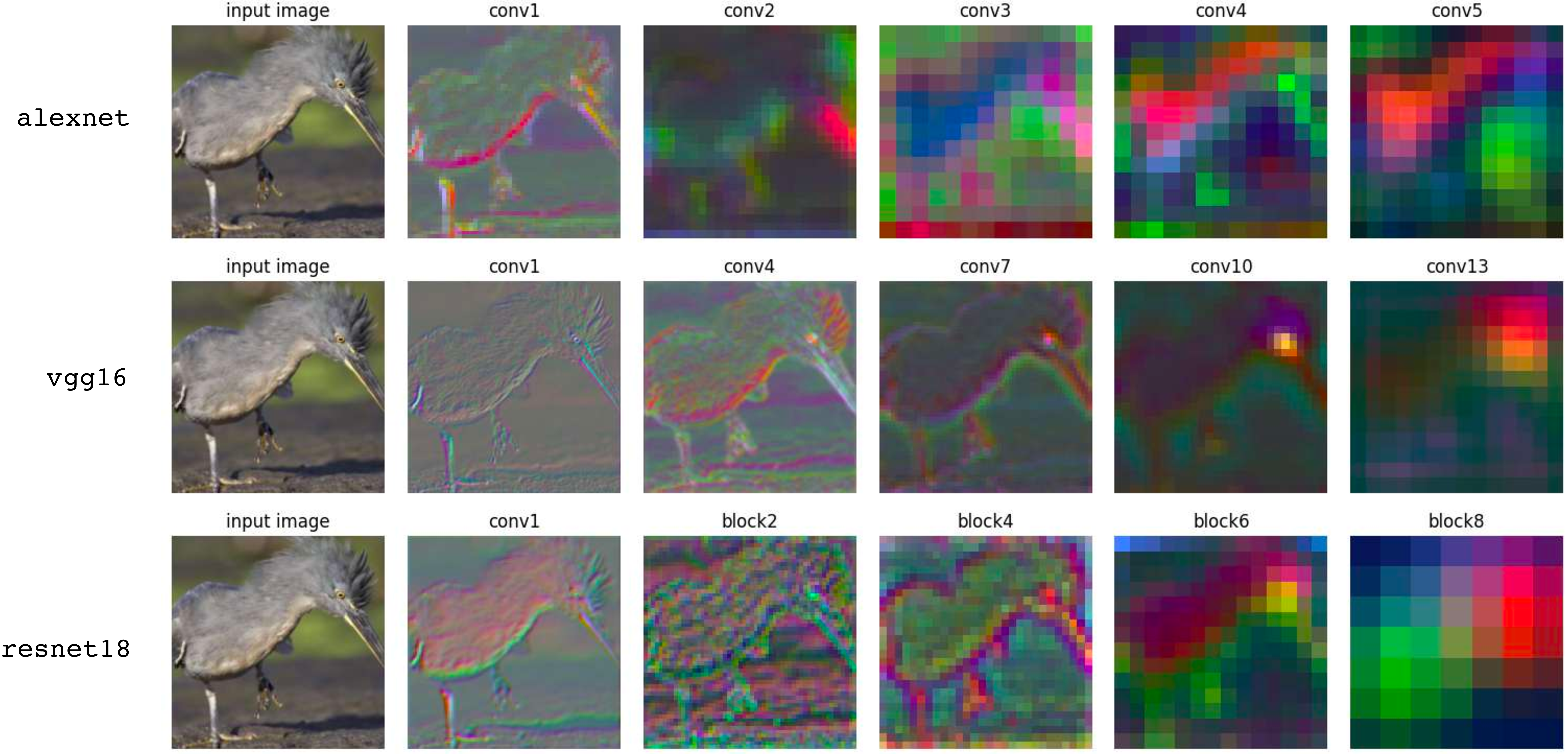
Figure 24.25 shows one more way to visualize feature maps. Rather than plotting the channels as a column of grayscale images, we run PCA to reduce the channel dimensionality to 3. Then we can directly render each feature map as a color image, with red showing the first priniciple component of each layer’s feature map, green the second, and blue the third. We show this for 5 layers in three common networks, AlexNet, VGG16 [2], and ResNet18 [3].
24.7 Receptive Fields
Receptive fields are another important concept when working with CNNs. In Chapter 1 we learned about history of receptive fields in neuroscience. As a reminder, the receptive field of a neuron is the region of the input signal that the neuron is sensitive to, i.e. its support. In multilayer perceptrons (MLPs, Chapter 12, the receptive field of each neuron is the entire input vector since MLPs use fully connected layers. In CNNs, on the other hand, each neuron only sees a portion of the input, since each output neuron on a conv layer is only connected to a subset of inputs to the conv layer, determined by the kernel size of the filter that produces that output.
The receptive fields of two example neurons in a CNN are shown below (Figure 24.26):

Notice that the receptive field grows the deeper we go into the network. To understand why, consider a CNN without nonlinearities. Then the \(l+1\)-th layer is the composition of \(l\) convolutional filters. As we saw in Section 15.4.1 composing filters results in a new filter with larger support (kernel size). The same happens in a CNN with pointwise nonlinearities, since pointwise operations do not affect receptive field (the outputs have the same receptive fields as the inputs). Further, whenever we have a downsampling layer by factor \(s\), the receptive field of the output is \(s\) times larger than the receptive field of the input. Because of these properties, receptive field sizes can grow rapidly as we go deeper in CNNs. Generally we want that the final layer of the CNN has large enough receptive fields to see entire input image, so that output neurons are sensitive to all pixels in the input. This can be achieved with a gap layer, whose output will always have a receptive field size that covers the entire input.
24.8 Spatial Outputs
In Section 24.4 we saw a CNN that outputs a single class probability vector for an image. What if we want to output a spatially varying map of predictions, like we discussed in the intro to this chapter? To achieve this, we can simply downsample less, so that the final layer of the CNN is a feature map that maintains higher spatial resolution.
It is also important to remove any global pooling layers.
An example is given below:
\[\begin{aligned} \mathbf{z}_1[c_1,:,:] &= \sum_{c=0}^2 \mathbf{w}_1[c,c_1,:,:] \star \mathbf{x} + b_1[c_1] &\triangleleft \quad \texttt{conv}\\ &&[3 \times N \times M] \rightarrow [C_1 \times N \times M]\nonumber\\ h[c_1,n,m] &= \max(z_1[c_1,n,m],0) &\triangleleft \quad \texttt{relu}\\ &&[C_1 \times N \times M] \rightarrow [C_1 \times N \times M]\nonumber\\ \mathbf{z}_2[c_2,:,:] &= \sum_{c_1=0}^{C_1-1} \mathbf{w}_2[c_1,c_2,:,:] \star \mathbf{x} + b_2[c_2] &\triangleleft \quad \texttt{conv}\\ &&[C_1 \times N \times M] \rightarrow [C_2 \times N \times M]\nonumber\\ y[k,n,m] &= \frac{e^{-\tau z_2[k,n,m]}}{\sum_{l=1}^K e^{-\tau z_2[l,n,m]}} &\triangleleft \quad \texttt{softmax}\\ &&[K \times N \times M] \rightarrow [K \times N \times M]\nonumber \end{aligned}\]
In Figure 24.27 we visualize this CNN (showing only a 1D slice of this 2D CNN):
Notation reminder: nodes that are squares indicate that they represent multiple channels (each is a vector of neurons)
Although historically CNNs first became popular as image classifiers, this usage hides their real power. Rather than thinking of them as image-to-label architectures, think of them as image-to-image architectures.
More generally, CNNs are \(\mathcal{X}\)-to-\(\mathcal{X}\) architectures for any domain \(\mathcal{X}\) over which translation can be defined.
24.9 CNN as a Sliding Filter
The core of CNNs are the convolutional layers, and in this section we will consider a CNN with only conv layers interleaved with pointwise nonlinearities. Such a CNN is sometimes called a fully convolutional network or FCN [4]. What we will show below is that a whole FCN is just another sliding image filter.
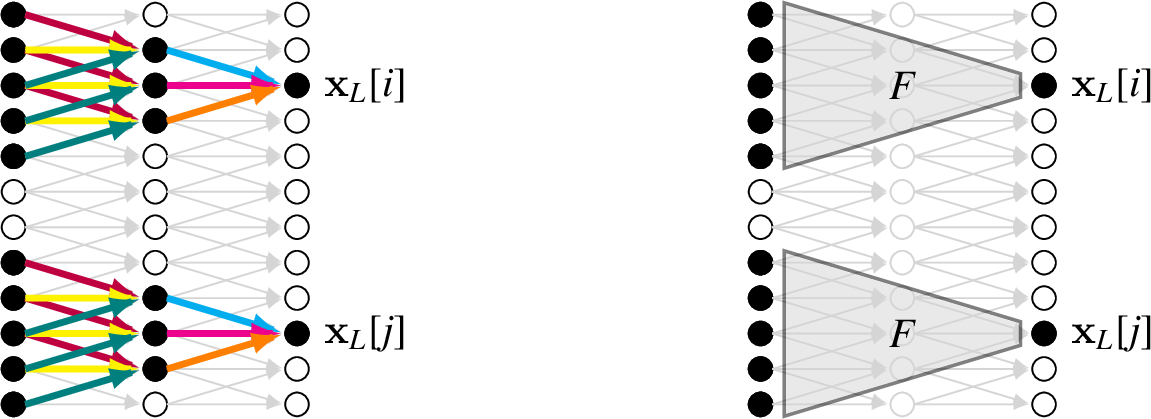
To see why, consider a CNN that processes a 1D signal, and outputs a feature map \(\mathbf{x}_L\). Take two feature vectors in the output map, \(\mathbf{x}_L[:,i]\) and \(\mathbf{x}_L[:,j]\). The feature vector at location \(i\) is some function, \(F\), of the input patch in its receptive field, \(\mathbf{x}_L[:,i] = F(\mathbf{x}_{\texttt{in}}[:,\texttt{RF}(i)])\), where \(\texttt{RF}\) returns the coordinates of the receptive field in the input image. It turns out that the feature vector at pixel \(j\) is produced by the same function, just applied to a different patch of the input: \(\mathbf{x}_L[:,j] = F(\mathbf{x}_{\texttt{in}}[:,\texttt{RF}(j)])\).
This is easiest to understand with a visual proof, which we give in Figure 24.28 (pointwise nonlinearities are omitted for clarity):
To understand this property, first imagine the CNN has no pointwise nonlinearities. Then the entire CNN is just the composition of a sequence of convolutions, which itself is a convolution (by Equation 15.5, convolving a signal with multiple filters in a row is equivalent to convolving the signal with a single equivalent filter). Therefore, a CNN with no nonlinearities is itself just a single big convolutional filter. The key property of such a system is that it processes each input patch independently and identically. Now notice that this key property is unchanged when we add pointwise nonlinearities, because they introduce no interaction between neurons or pixels (they are pointwise after all). Hence it follows that a complete CNN, made up only of convolutional layers and pointwies nonlinearities, is itself a nonlinear operator that applies the same transformation independently and identically to each patch of the input signal, i.e. a nonlinear filter!
This is why, in the intro to this chapter, we visualized a CNN as chopping up an image into patches and applying the same “classifier” function to each patch.
24.10 Why Process Images Patch by Patch?
As we have seen above, a fully convoutional CNN can be thought of a function that processes each patch of the input independently and identically.
A CNN is a non-linear filter. Edge colors indicate shared weights; two edges with the same color have the same weight. The colors demonstrate that the same function \(F\) is applied to each patch of input nodes.
In this section we will discuss why these two properties are useful for image processing.
Property #1: Treating Patches as Independent
This is a divide-and-conquer strategy. If you were to try to understand a complex problem, you might break it up into small pieces and solve each one separately. That’s all a CNN is doing. We split up a big problem (i.e. “interpret this whole photo”) into a bunch of smaller problems (i.e. “interpret each small patch in the image”).
Why is this a good strategy?
The small problems are easier to solve than the original problem.
The small problems can all be solved in parallel.
This approach is agnostic to signal length, that is, you can solve an arbitrarily large problem just by breaking it down to bite size pieces and solving them “bird by bird” [5].
Chopping up into small patches like this is sufficient for many vision problems because the world exhibits locality: related things clump together, that is, within a single patch; far apart things can often be safely assumed to be independent.
Property #2: Processing Each Patch Identically
For images, convolution is an especially suitable strategy because visual content tends to be translation invariant, and, as we learned in previous chapters, the convolution operator is also translation invariant.
Typically, objects can appear anywhere in an image and look the same, like the birds in the photo from Figure 24.1. This is because as the birds fly across the frame their position changes but their identity and appearance does not. More generally, as a camera pans across a scene, the content shifts in position but is otherwise unchanged.
Because the visual world is roughly translation invariant, it is justified to process each patch the same way, regardless of its position (i.e., its translation away from some canonical center patch).
Translation invariant just means we process each patch identically, using the same function \(f\). Some texts instead use the term to describe convolutions. This places emphasis on the fact that if we shift the input signal by some translation, then the output signal will get shifted by the same amount. That is, if \(f\) is a convolution, we have the property:
\[\begin{aligned} f(\texttt{translate}(\mathbf{x})) = \texttt{translate}(f(\mathbf{x})) \end{aligned}\]
24.11 Popular CNN Architectures
We have now seen all the essential building blocks of CNNs. In this section we will treat these blocks like LEGOs and show how to piece them together to make a variety of useful architectures.
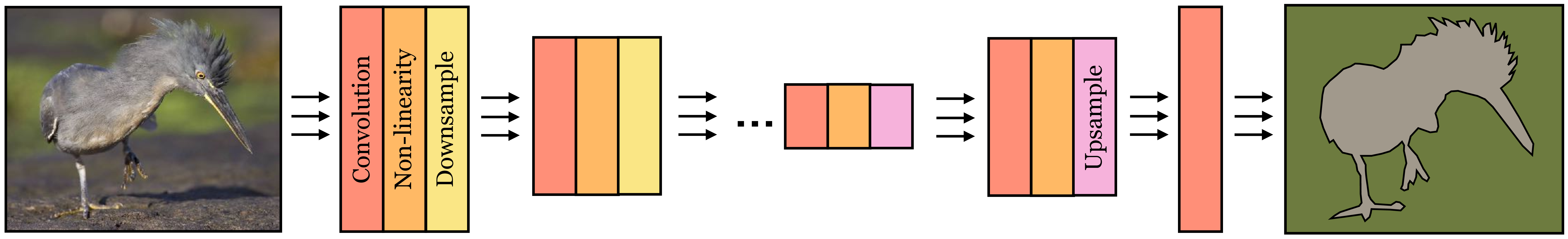
24.11.1 Encoder and Decoders
In Chapter 23, we encountered image pyramids that include both an analysis pipeline, which converts an image into a multiscale representation of filter responses, and a synthesis pipeline, which reconstructs the image from the filter responses. Deep networks also may operate in either the analysis direction or the synthesis direction. In the context of deep networks, we call the analysis network an encoder and the synthesis network a decoder. An encoder maps from data to a representation of that data, which is usually lower dimensional, and a decoder performs the inverse operation, mapping from a representation back to the data.
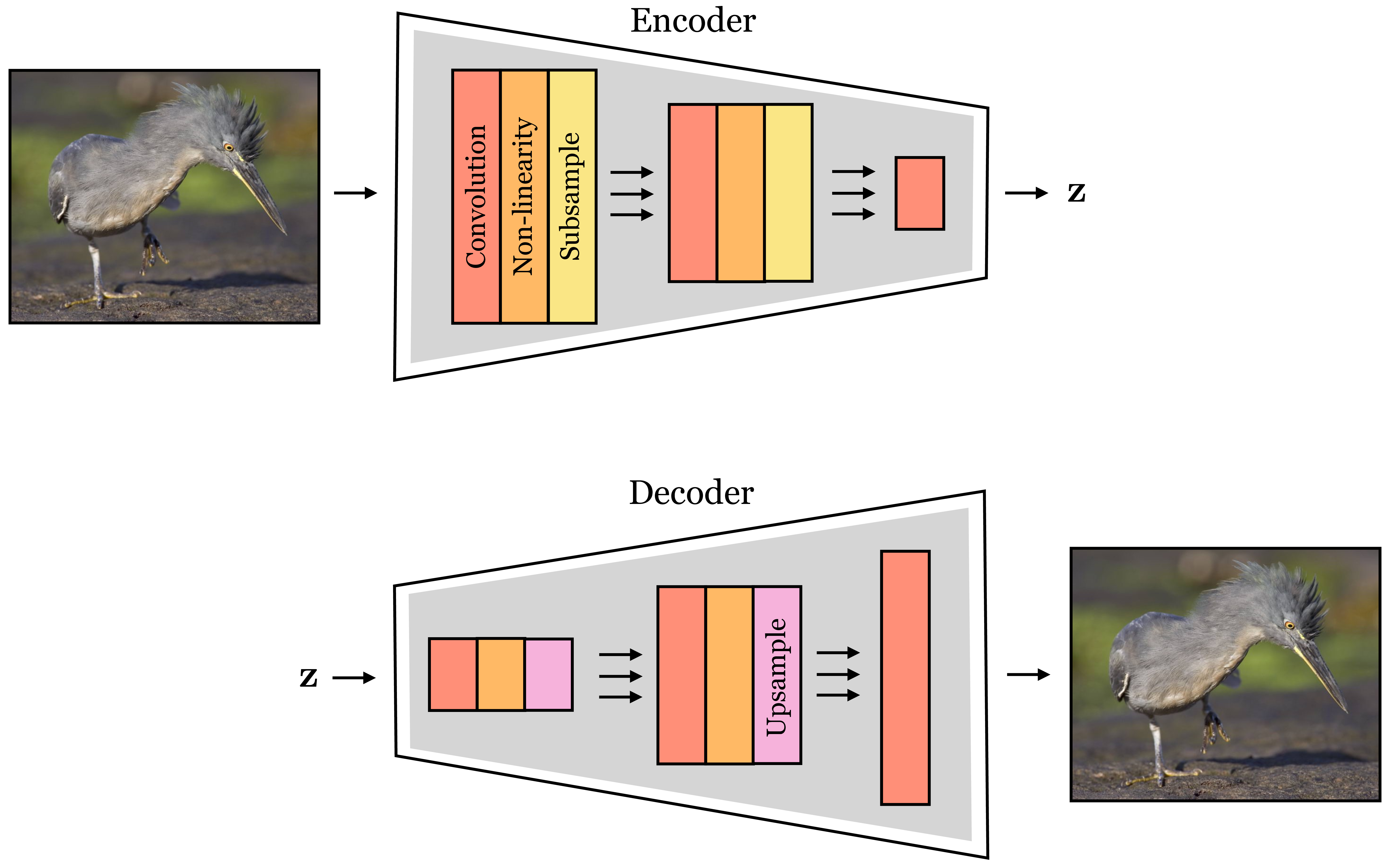
Encoder and decoder networks will appear many times in this book, and can be made from many different architectures, including those that are not neural nets. In the context of CNNs, encoders are typically nets that take an image as input and then downsample it, layer by layer, until producing a much lower-dimensional feature map as output. A decoder is the opposite, taking a set of low-dimensional features as input, then upsampling them, layer by layer, until producing an image as the final output. An example of an encoder is an image classifier and an example of a decoder is an image generator (covered in Chapter 32. These two architectural patterns are shown in Figure 24.29.
One powerful thing you can do with encoders and decoders is to put them together, forming an encoder-decoder. Such an architecture first encodes the input image into a low-dimensional representation, then decodes the representation back into an image output. This is therefore a suitable architecture for image-to-image problems, and it has a few advantages over the image-to-image CNNs we saw in Section 24.8: 1) by downsampling, the internal feature maps are smaller, using less memory and computation, 2) encoder-decoders introduce an information bottleneck – i.e. the representation between the encoder and decoder is low-dimensional and can only transmit so much information – and this forces abstraction. This latter concept is one we will study in much greater detail in Chapter 30, where we will see several benefits of compressing a signal. A schematic of the encoder-decoder architecture is shown in Figure 24.30.
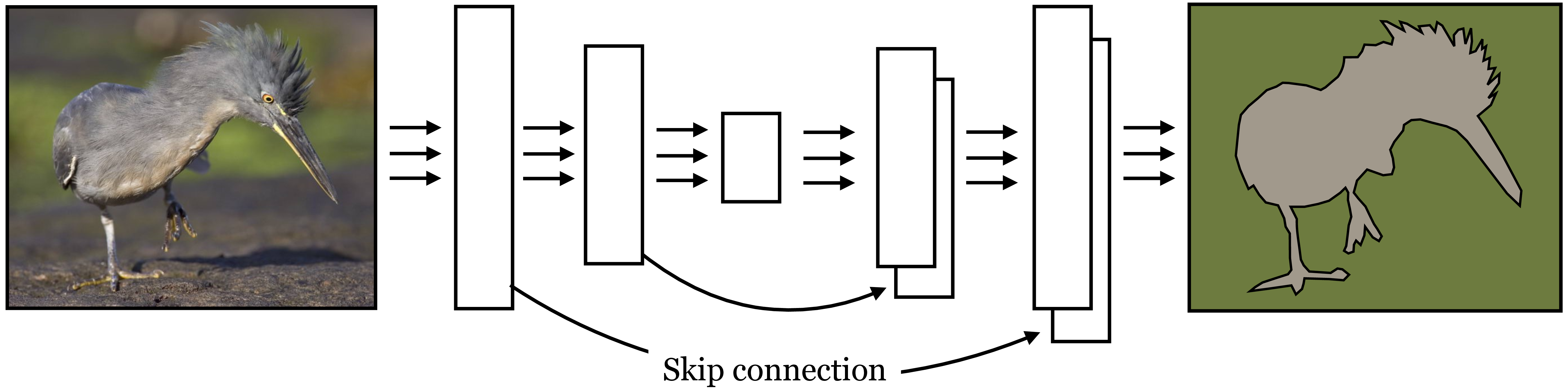
24.11.2 U-Nets
Encoder-decoders force the signal to pass through a bottleneck, and although this can be a good thing (as discussed above), it also makes the task of the decoder rather difficult. In particular, the decoder may fail to be able to output high frequency details; for a semantic segmentation network, the consequence could be that the predicted label map is very coarse.
To circumvent this problem, we can add that shuttle information directly across blocks of layers in the net. A skip connection \(f\) is simply an identity pathway that connects two disparate layers of a net, \(f(\mathbf{x}) = \mathbf{x}\).
Adding skip connections to an encoder-decoder results in an architecture known as a U-Net [6]. In this architecture, skip connections are arranged in a mirror pattern, where layer \(l\) is connected directly to layer \((L-l)\). The output of a skip connection must somehow be reintegrated into the network. U-nets do this by concatenating the activations from the prior layer to the activations on the later layer, along the channel dimension. This architecture can maintain the information-bottleneck of the encoder-decoder, with its incumbent benefits in terms of memory and compute efficiency and forced abstraction, while also allowing residual information to flow through the skip connections, thereby not sacrificing the ability to output high-frequency spatial predictions. U-Nets look a lot like the steerable pyramids from Chapter 23, which also consistent of a downsampling analysis path followed by an upsampling synthesis path, with skip connections in between mirror image stages in the pathways. The main difference is that the U-Net has learned filters and nonlinearities. A schematic of a U-net is given in Figure 24.31.
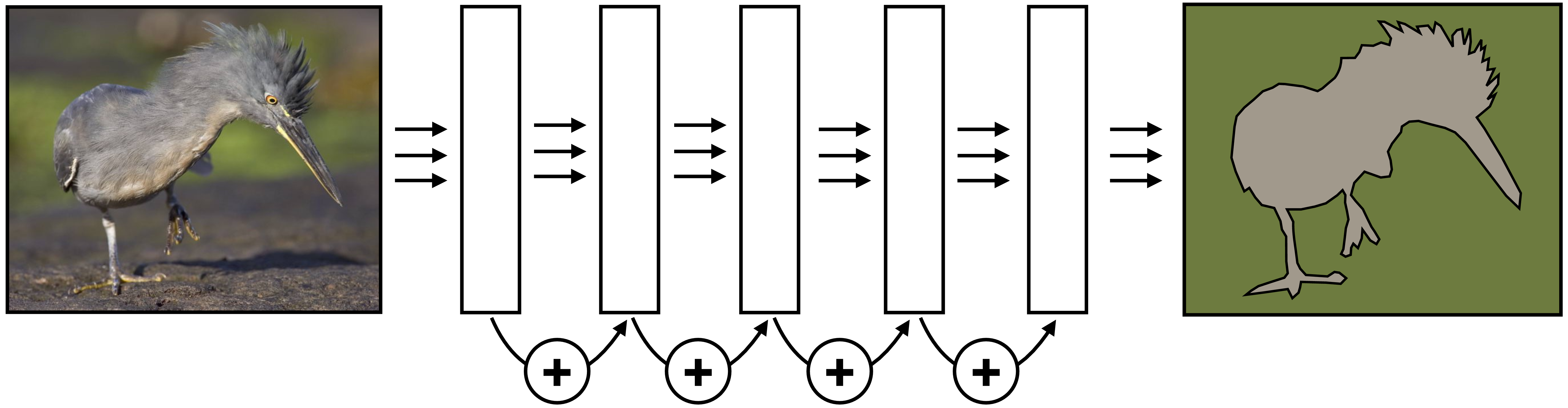
24.11.3 ResNets
Another popular architecture that uses skip connections is called Residual Networks or ResNets [3].
See also Highway Networks [7], a related architecture that uses a form of skip connection but controlled by multiplicative gates.
In the context of ResNets, skip connections are called residual connections. This kind of skip connection is added to the output of a block of layers \(F\): \[\begin{aligned} \mathbf{x}_{\texttt{out}}= F(\mathbf{x}_{\texttt{in}}) + \mathbf{x}_{\texttt{in}}\quad\quad \triangleleft \quad \texttt{residual block} \end{aligned}\]
In a residual block like this, you can think of \(F\) as a residual that additively perturbs \(\mathbf{x}_{\texttt{in}}\) to transform it into an improved \(\mathbf{x}_{\texttt{out}}\). If \(\mathbf{x}_{\texttt{out}}\) does not have the same dimensionality as \(\mathbf{x}_{\texttt{in}}\), then we can add a linear mapping to convert the dimensions: \(\mathbf{x}_{\texttt{out}}= F(\mathbf{x}_{\texttt{in}}) + \mathbf{W}\mathbf{x}_{\texttt{in}}\).
It is easy for a residual block to simply perform an identity mapping, it just has to learn to set \(F\) to zero. Because of this, if we stack many residual blocks in a row, it can end up that the net learns to use only a subset of them. If we set the number of stacked residual blocks to be very large then the net can essentially learn how deep to make itself, using as many blocks as necessary to solve the task. ResNets often exploit this fact by being very deep; for example, they may be hundreds of blocks deep. Figure 24.32 depicts a 5 block deep ResNet.
24.12 Concluding Remarks
We will see in later chapters that several new kinds of models are recently supplanting CNNs as the most successful architectures for vision problems. One such architecture is the transformer Chapter 26. It may be tempting to think, “Why did we bother learning about CNNs then, if transformers are better!” The reason we cover CNNs is not because the exact architecture presented here will last, but because the underlying principles it embodies are ubiquitous in sensory processing. The two key properties mentioned in Section 24.10 are in fact present in transformers and many other architectures beyond CNNs: transformers also include stages that process each patch identically and independently, but they interleave these stages with other stages that globalize information across patches. It comes down to preferences whether you want to call these newer architectures convolutional or not, and there is currently some debate about it in the community. For us it doesn’t matter, because if we learn the principles we can recognize them in all the systems we encounter and need not get hung up on names.