49 Learning to Estimate Motion
49.1 Introduction
We have discussed in the previous sections a number of model-based methods for motion estimation. If these models describe the equations of motion based from first principles, why is that we need learning based methods at all? The reason is that the models make a number of assumptions that are not always true. Also, there are other sources of information that can reveal properties about motion that cannot be modeled but that can be learned.
Causes of modeling errors include failure of the brightness constancy assumption; the presence of occlusions, shadows and changes in illumination; new structures appearing due to changes in the resolution as a result of motion, deformable surfaces; and so on. Many of the motion computations involved approximations such as approximating the derivatives with finite size discrete convolutions. There could also be other motion-relevant cues present in the image, such as monocular depth cues that provide information about the three-dimensional (3D) scene structure and the presence of familiar objects for which we can have strong priors about their motion. These could include that buildings do not move, walls are solid and usually featureless, people are deformable, trees leaves have huge number of occlusions, and so on. Those semantic properties can be implicitly exploited by a learning-based model.
49.2 Learning-Based Approaches
Learning-based approaches rely on many of the concepts we introduced in the previous chapters. We will differentiate between two big families of models: supervised models that learn to estimate motion using a database of training examples, and unsupervised models that learn to estimate motion without training data.
49.2.1 Supervised Models for Optical Flow Estimation
The simplest formulation for learning to estimate optical flow is when we have available a dataset of image sequences with associated ground truth optical flow. Researchers have used synthetic data [1], using lidar [2] or human annotations [3] to build datasets with ground truth motion. In previous approaches, ground truth data could be used for evaluation; however, we will use it here to train a model to predict motion directly from the input frames.
49.2.1.1 Architectures
As in the case of stereo, we can train a function to estimate optical flow from two frames:
\[\left[ \hat{\mathbf{u}}, \hat{\mathbf{v}} \right] = h_\theta \left( \boldsymbol\ell_1, \boldsymbol\ell_2 \right)\] One of the first approaches to use this formulation with neural networks was FlowNet [4]. The architecture is simple.
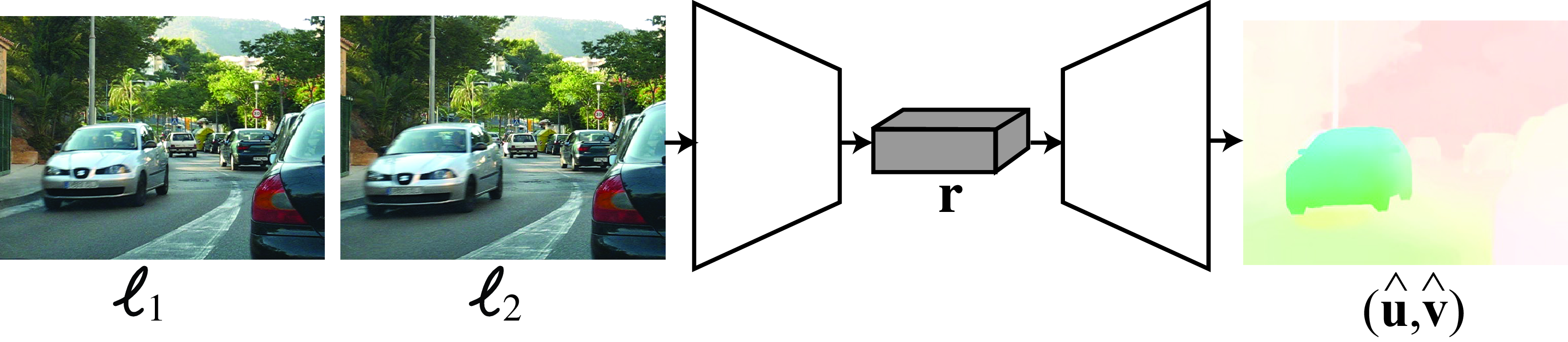
The direct approach depicted in Figure 49.1 learns to estimate optical flow directly from a pair of frames. This architecture makes no assumptions about which architectural priors are needed to compute optical flow from images. The architecture is trained end-to-end using ground truth optical flow.
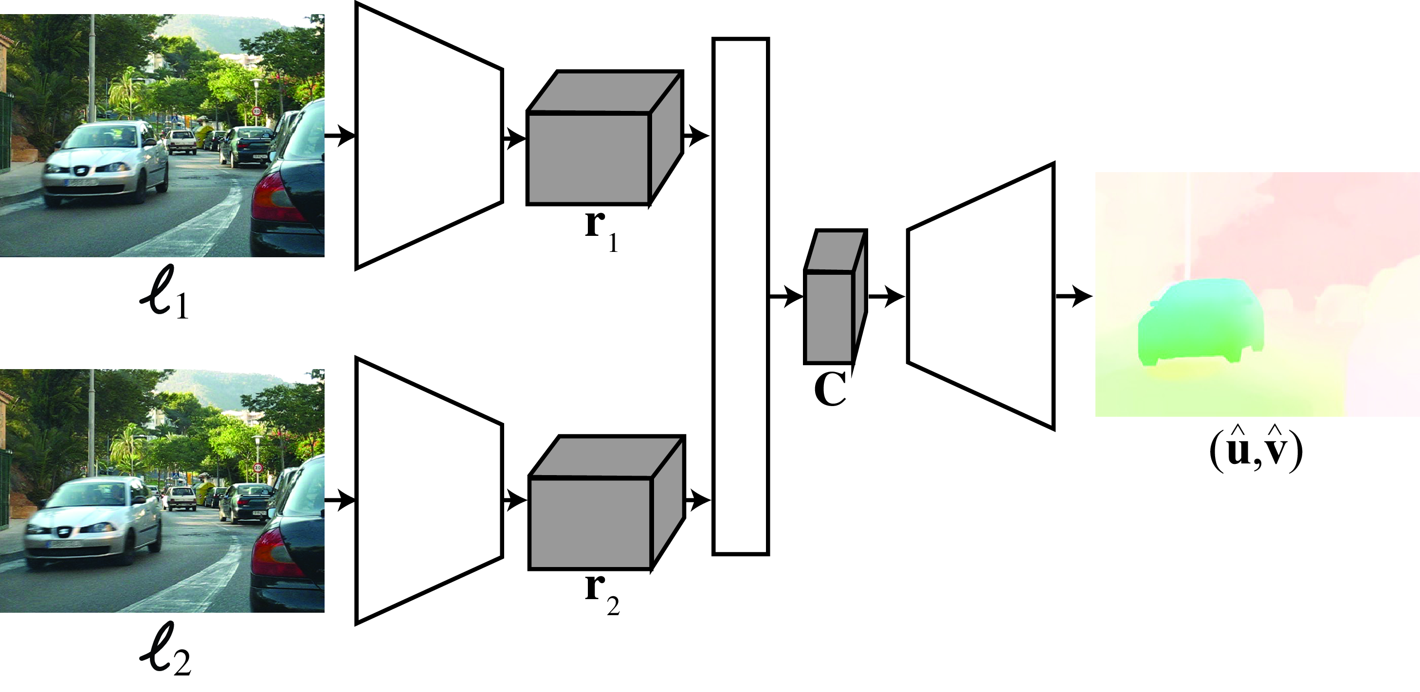
Another common approach, depicted in the block diagram shown in Figure 49.2, is to define an architecture that follows the same steps as traditional approaches:
Extract features from each image using a pair of networks with shared weights. This can be done by a feature pyramid [5].
Form a 3D cost volume indicating the local visual evidence of a match between the two images for each possible pixel position. This 3D cost volume can be referenced to the \(H\) and \(V\) positions of one of the input images (generally the first frame is the reference frame).
Train and apply a CNN to aggregate (process) the costs over the cost volume in order to estimate a single best optical flow for each pixel position.
Use a coarse-to-fine estimation procedure where optical flow estimated at a coarse scale is used to warp the features at a finer scale to compute a refined cost volume. Then, estimate an update to the optical flow to warp the features and the next finer level of the pyramid.
Other variations over this architecture incorporate some of the concepts we studied before, such as coarse-to-fine refinement, matching, and smoothing. Different approaches will differ in some of the details of how each step is implemented and how training takes place. The main building blocks can be implemented with convolutional neural networks or transformers. The main difference between the matching-based and gradient-based methods described earlier is that instead of using predefined functions, the architectures are trained end-to-end to minimize the optical flow error when compared with ground truth data.
49.2.1.2 Loss functions
In supervised optical flow estimation, the most common loss is the endpoint error, which is the average, over the whole image, if the distance between the estimated optical flow vector, \((\hat{u},\hat{v})\) and the ground-truth vector, \((u,v)\): \[\mathcal{L} \left( \hat{\mathbf{u}}, \hat{\mathbf{v}}, \mathbf{u}, \mathbf{v} \right) = \sum_{n,m} (\hat{u}[n,m] - u[n,m])^2 + (\hat{v}[n,m] - v[n,m])^2\] The sum is over all the pixels in the image. Each pixel has an estimated optical flow \((\hat{u}[n,m],\hat{v}[n,m])\).

49.2.1.3 Handling occlusions
One of the challenges for estimating optical flow is that, as objects move, they will occlude some pixels from the background and reveal new ones. Therefore, together with the estimated flow it is also convenient to detect occluded pixels. If we have ground truth data, we can train a function to estimate optical flow and the occlusion map from two frames: \[\left[ \hat{\mathbf{u}}, \hat{\mathbf{v}}, \hat{\mathbf{o}} \right] = h_\theta \left( \boldsymbol\ell_1, \boldsymbol\ell_2 \right)\]
49.2.1.4 Training set
The biggest challenge of using a supervised model for motion estimation is that ground truth data is very hard to collect. This is probably one of the main limitations of these approaches. There are some small existing datasets, although this might change in a few years.
The largest existing datasets are synthetic 3D scenes with moving objects that can be rendered, which will give us perfect ground truth data to train the regression function. There are several examples of existing datasets such as this, like the Middelbury dataset [6], which contains six real and synthetic sequences with ground truth optical flow. The optical flow for the real sequences was obtained by tracking hidden fluorescent texture. The KITTI dataset [2] contains real motion recorded from a moving car. The MPI Sintel [1] contains synthetic sequences made with great effort to make the scenes look realistic. Finally, the Flying Chairs dataset is an interesting synthetic dataset that consists of pasting the image of a random number of chairs over a background image [4]. Motion is created by applying different affine transformations to the background and the chairs. These sequences are easy to generate and pay little attention to their realism. This makes it possible to generate a very large number of sequences for training, allowing for competitive performance when used to train a neural network.
49.2.2 Unsupervised Learning of Optical Flow
Collecting ground truth data is the Achilles heel for learning-based approaches. This is particularly true for optical flow as it can not be recorded directly. Ground truth data optical flow can be obtained on synthetic data only, and for real data one needs to create specific recording scenarios that allow inferring accurate optical flow or relying on noisy human annotations [3]. As a consequence, real data collection is expensive and nonscalable.
Is it possible to learn to estimate optical flow by just looking at movies without using ground truth data?
Unsupervised methods for training an optical flow model will make some assumptions about dynamic image formation. Those assumptions will be similar to the ones we have presented all along this chapter- (1) when the motion is due only to camera motion, the optical flow will have to fit the equations of the projected motion that provide constraints that can be used to train a model; (2) we can assume that the appearances of objects and surfaces in the scene do not change due to motion (brightness constancy assumption); and (3) we can expect the optical flow to be smooth over regions, although with sharp variations along occlusion boundaries.
One typical formulation consists in learning to predict the displacement from frame 1 to frame 2, so that if we warp frame 1 we minimize the reconstruction error of frame 2. This is achieved by using the photometric loss:
\[L_{photo}(\boldsymbol\ell_1,\boldsymbol\ell_2,\mathbf{u}, \mathbf{v})= \sum_{x,y} \left| \ell_2 (x+\hat{u},y+\hat{v}) - \ell_1 (x,y)) \right| ^2\] where now \(\left[ \hat{\mathbf{u}}, \hat{\mathbf{v}} \right] = h_\theta \left( \boldsymbol\ell_1, \boldsymbol\ell_2 \right)\).
The learning is done by searching over the parameter space for the parameters \(\theta\) that minimize the photometric loss over a large collection of videos. The photometric loss can also be replaced by the L1 or other robust norms. If the network also predicts occlusions, the photometric loss can include a weight that cancels the contribution of occluded pixels to the loss.
The network can also take as input multiple frames and not just two.
49.3 Concluding Remarks
Supervised and unsupervised learning-based methods are now the state-of-the-art in motion estimation. But an accurate solution is still missing. One important question is, do we really need learning in order to solve this problem? Should we abandon the derivation of physically motivated algorithms for motion estimation that require no training? Our answer is that we should pursue both directions of work.