29 Probabilistic Graphical Models
29.1 Introduction
Probabilistic graphical models describe joint probability distributions in a modular way that allows us to reason about the visual world even when we’re modeling very complicated situations. These models are useful in vision, where we often need to exploit modularity to make computations tractable.
A probabilistic graphical model is a graph that describes a class of probability distributions sharing a common structure. The graph has nodes, drawn as circles, indicating the variables of the joint probability. It has edges, drawn as lines connecting nodes to other nodes. At first, we’ll restrict our attention to a type of graphical model called undirected, so the edges are line segments without arrowheads.
In undirected graphical models, the edges indicate the conditional independence structure of the nodes of the graph. If there is no edge between two nodes, then the variables described by those nodes are independent, conditioned on the values of intervening nodes in any path between them in the graph. If two nodes do have a line between them, then we cannot assume they are independent. We introduce this through a set of examples.
29.2 Simple Examples
Here is the simplest probabilistic graphical model:
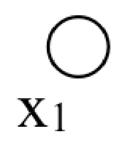
This graph is just a single node for the variable \(x_1\). There is no restriction imposed by the graph on the functional form of its probability function. In keeping with notation we’ll use later, we write that the probability distribution over \(x_1\), \(p(x_1) = \phi_1(x_1)\).
Another trivial graphical model is this:

Here, the lack of a line connecting \(x_1\) with \(x_2\) indicates a lack of statistical dependence between these two variables. In detail, we condition on knowing the values of any connecting neighbors of \(x_1\) and \(x_2\) (in this case there are none) and thus \(x_1\) and \(x_2\) are statistically independent. Because of that independence, the joint probability depicted by this graphical model must be a product of each variable’s marginal probability and thus must have the form: \(p(x_1, x_2) = \phi_1(x_1) \phi_2(x_2)\).
Let’s add a line between these two variables:
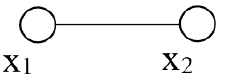
By that graph, we mean that there may be a statistical dependency between the two variables. The class of probability distributions depicted here is now more general than the one above, and we can only write that the joint probability as some unknown function of \(x_1\) and \(x_2\), \(p(x_1, x_2) = \phi_{12}(x_1, x_2)\). This graph offers no simplification from the most general probability function of two variables.
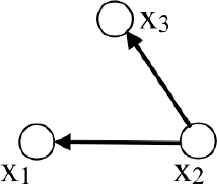
Here is a graph with some structure:
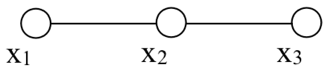
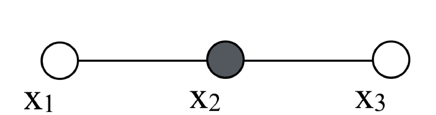
This graph means that if we condition on the variable \(x_2\), then \(x_1\) and \(x_3\) are independent. A general form for \(p(x_1, x_2, x_3)\) that guarantees such conditional independence is \[p(x_1, x_2, x_3) = \phi_{12}(x_1, x_2) \phi_{23}(x_2, x_3). \tag{29.1}\] Note the conditional independence implicit in equation (Equation 29.1): if the value of \(x_2\) is given (indicated by the solid circle in the graph below), then the joint probability of equation (Equation 29.1) becomes a product of some function \(f(x_1)\) times some other function \(g(x_3)\), revealing the conditional independence of \(x_1\) and \(x_3\). Graphically, we denote the conditioning on the variable \(x_2\) with a filled circle for that node:
We will exploit that structure of the joint probability to perform inference efficiently using an algorithm called belief propagation (BP).
A celebrated theorem, the Hammersley-Clifford theorem [1], tells the form the joint probability must have for any given graphical model. The joint probability for a probabilistic graphical model must be a product of functions of each the maximal cliques of the graph. Here we define the terms.
A clique is any set of nodes where each node is connected to every other node in the clique. These graphs illustrate the clique property:
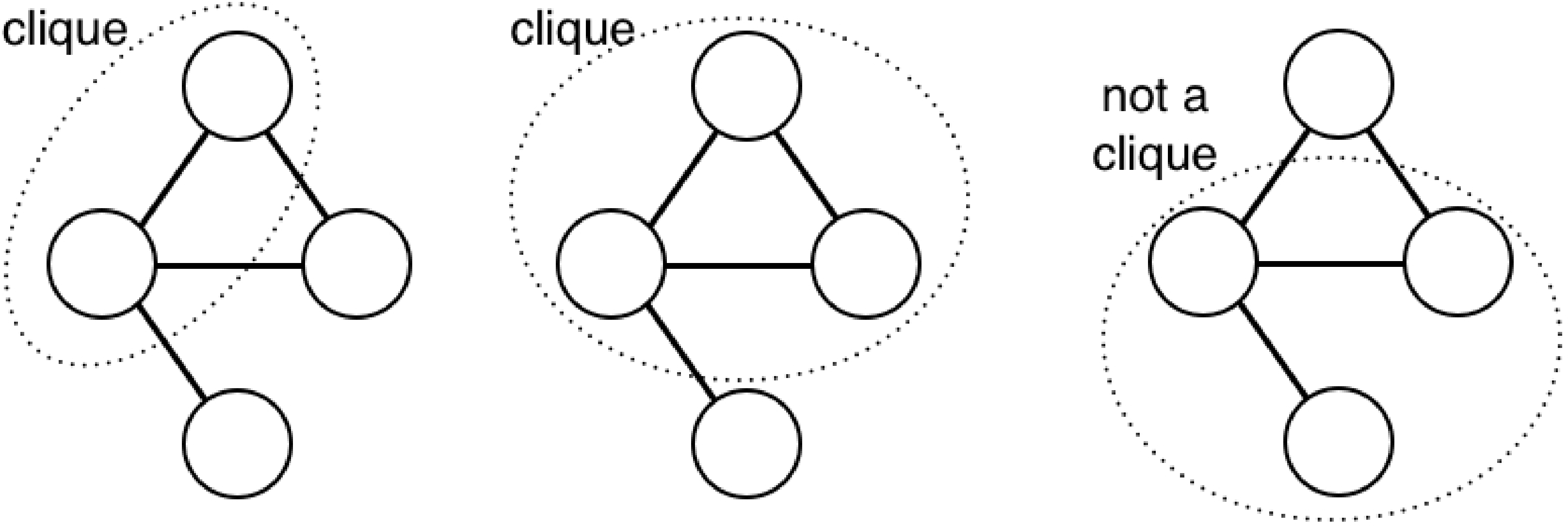
A maximal clique is a clique that can’t include more nodes of the graph without losing the clique property. The sets of nodes below form maximal cliques (left), or do not (right):

The Hammersley-Clifford theorem [1] states that a positive probability distribution has the independence structure described by a graphical model if and only if it can be written as a product of functions over the variables of each maximal clique: \[p(x_1, x_2, \ldots, x_N) = \prod_{x_c \in x_i} \Psi_{c} (x_c),\] where the product is over all maximal cliques \(x_c\) in the graph, \(x_i\).
In the example of graph in Figure 29.1, the maximal cliques are (x1, x2) and (x2, x3), so the Hammersley-Clifford theorem says that the corresponding joint probability must be of the form of equation (Equation 29.1).
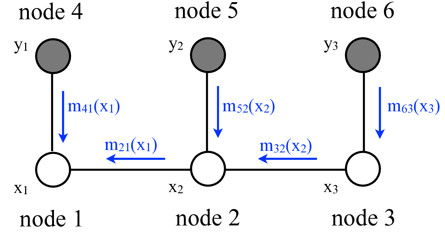
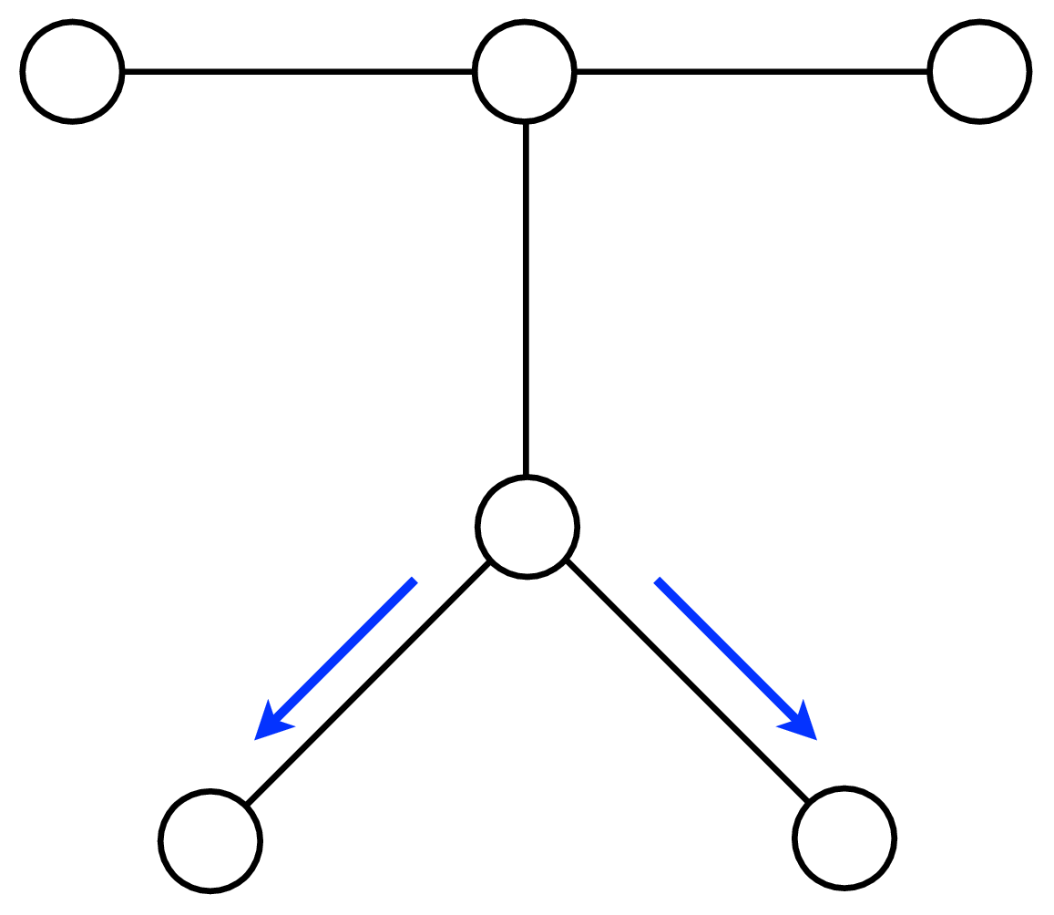
Now we examine some graphical model structures that are especially useful in vision. In perception problems, we typically have both observed and unobserved variables. The graph below shows a simple Markov chain [2] structure with three observed variables, shaded, labeled \(y_i\), and three unobserved variables, labeled \(x_i\):
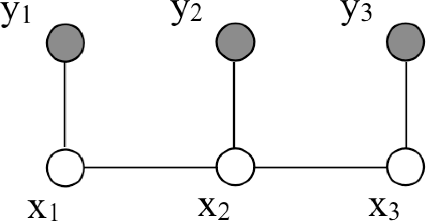
This is a chain because the variables form a linear sequence. It’s a Markov chain structure because the hidden variables have the Markov property: conditional on \(x_2\), variable \(x_3\) is independent of variable \(x_1\). The joint probability of all the variables shown here is \(p(x_1, x_2, x_3, y_1, y_2, y_3) = \phi_{12}(x_1, x_2) \phi_{23}(x_2, x_3) \psi_{1}(y_1, x_1) \psi_{2}(y_2, x_2) \psi_{3}(y_3, x_3)\). Using \(p(a,b) = p(a \bigm | b) p(b)\), we can also write the probability of the \(x\) variables conditioned on the observations \(y\), \[p(x_1, x_2, x_3 \bigm | y_1, y_2, y_3) = \frac{1}{p(\mathbf{y})} \phi_{12}(x_1, x_2) \phi_{23}(x_2, x_3) \psi_{1}(y_1, x_1) \psi_{2}(y_2, x_2) \psi_{3}(y_3, x_3).\] For brevity, we write \(p(\mathbf{y})\) for \(p(y_1, y_2, y_3)\). Thus, to form the conditional distribution, within a normalization factor, we simply include the observed variable values into the joint probability. For vision applications, we often use such Markov chain structures to describe events over time.
To capture relationships over space, a two-dimensional (2D) structure is useful, called a Markov random field (MRF) [3]:
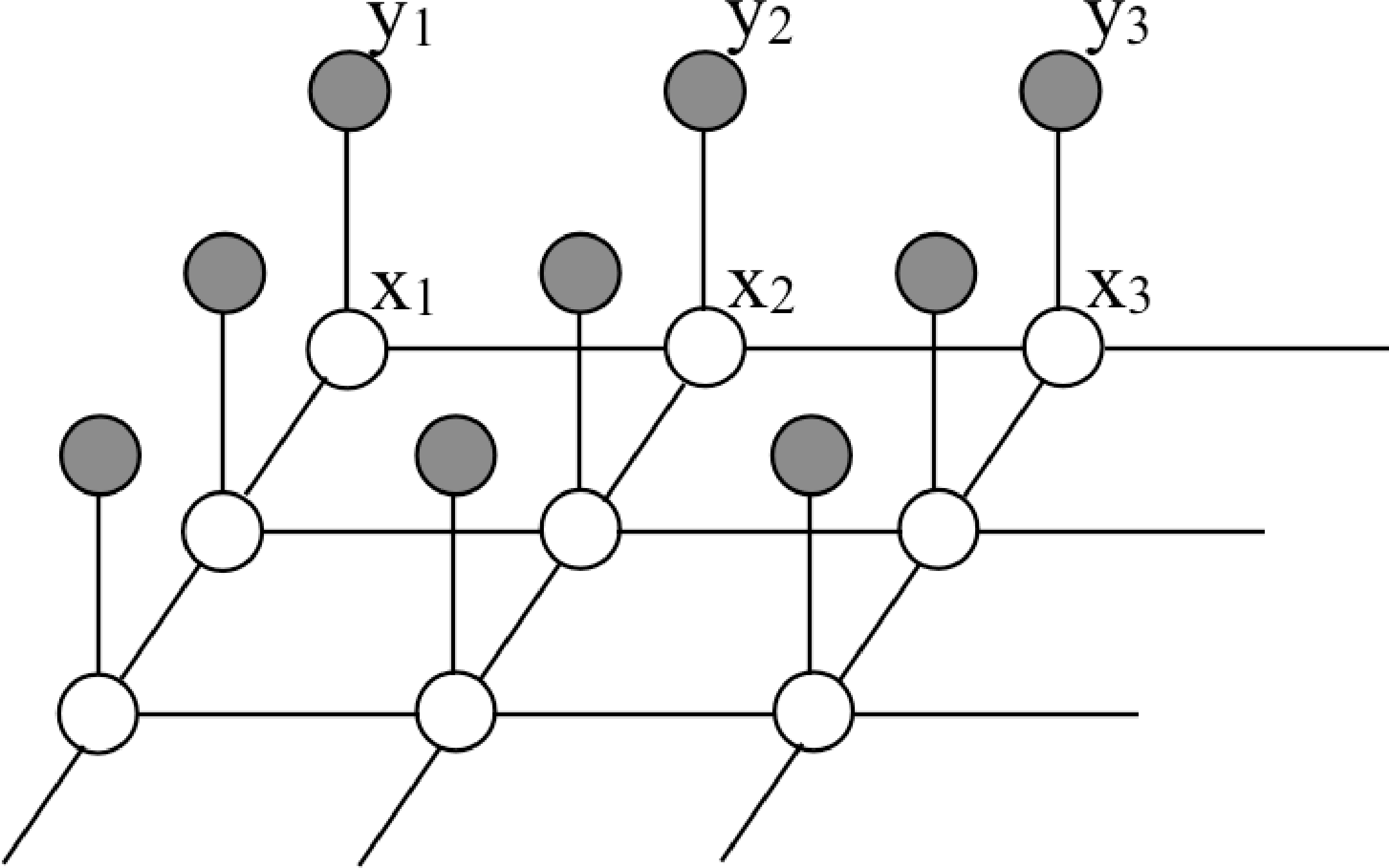
Then the joint probability over all the variables factorizes into this product:
\[p(\mathbf{x} \bigm | \mathbf{y}) = \frac{1}{p(\mathbf{y})} \prod_{(i,j)} \phi_{ij}(x_i, x_j) \prod_i \psi_i(x_i, y_i),\] where the first product is over all spatial neighbors \(i\) and \(j\), and the second product is over all nodes \(i\).
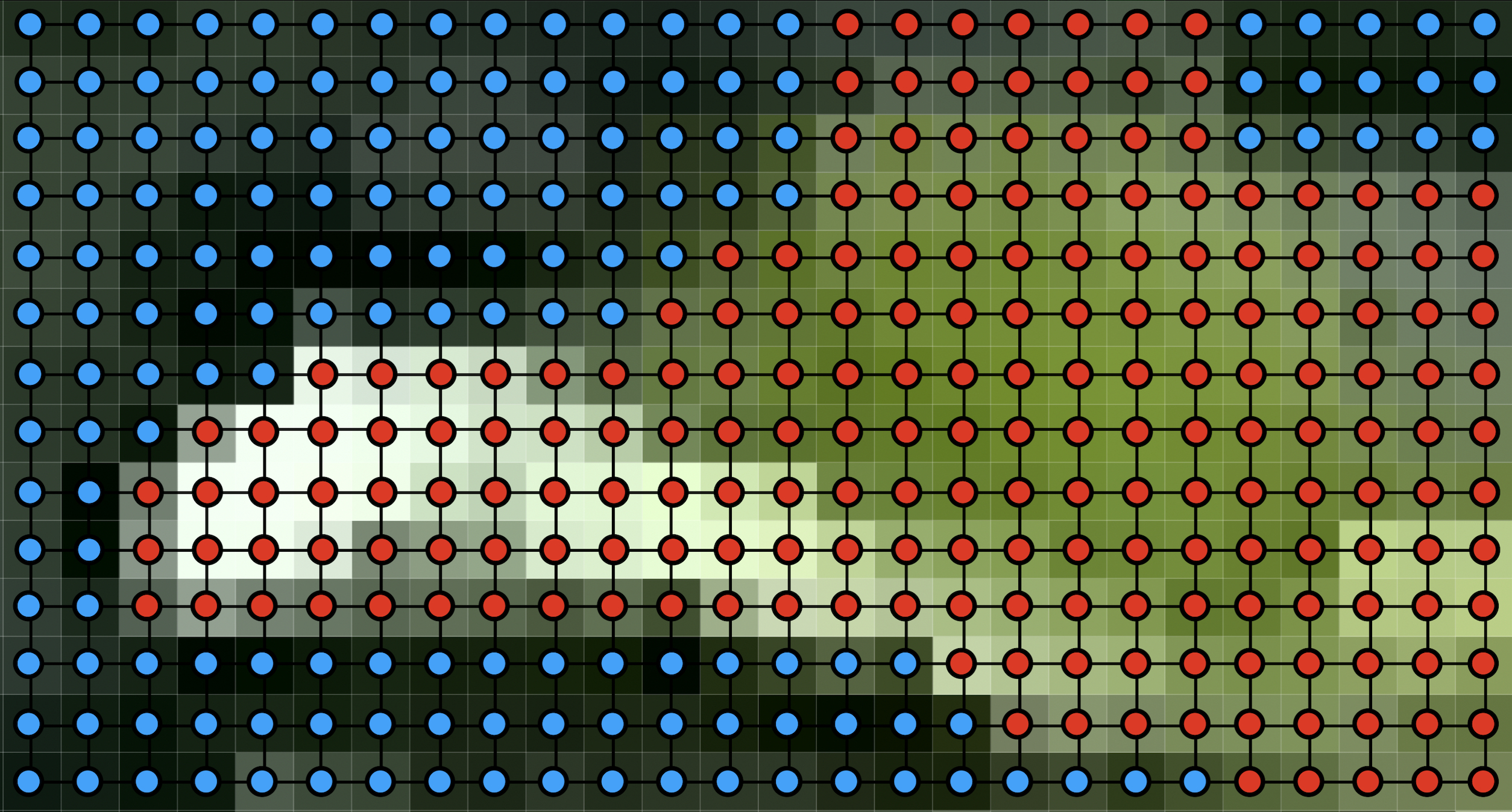
An example of how Markov random field models are applied to images is depicted in Figure 29.4, which show a small image region and its context in the image (Figure 29.4). Figure 29.4 shows an MRF with each node corresponding to a pixel of the image region. The states of an MRF can be indicator variables of image segment membership for each pixel. The states of a hypothetical most-probable configuration of this MRF are shown as the color of each node in this illustration.
29.3 Directed Graphical Models
In addition to undirected graphical models, another type of graphical model is commonly used. Directed graphical models [4] describe factorizations of the joint probability into products of conditional probability distributions. Each node in a directed graph contributes a well-specified factor in the joint probability: the probability of its variable, conditioned on all the variables originating arrows pointing into it. So this graph
denotes the joint probability, \[p(x_1, x_2, x_3) = p(x_2) p(x_1 \bigm | x_2) p(x_3 \bigm | x_2) \tag{29.2}\]
The general rule for writing the joint probability described by a directed graph is this: Each node, \(x_n\), contributes the factor \(p(x_n \bigm | x_{\Xi})\), where \(\Xi\) is the set of nodes with arrows pointing in to node \(x_n\). You can verify that equation (Equation 29.2) follows this rule. Directed graphical models are often used to describe causal processes.
29.4 Inference in Graphical Models
Given a probabilistic graphical model and observations, we want to estimate the states of the unobserved variables. For example, given image observations, we may want to estimate the pose of the person. The belief propagation algorithm lets us do that efficiently.
Recall the Bayesian inference task: our observations are the elements of a vector, \(\mathbf{y}\), and we seek to infer the probability \(p(\mathbf{x} \bigm | \mathbf{y})\) of some scene parameters, \(\mathbf{x}\), given the observations. By Bayes’ theorem, we have \[p(\mathbf{x} \bigm | \mathbf{y}) = \frac{p(\mathbf{y} \bigm | \mathbf{x}) p(\mathbf{x}) }{p(\mathbf{y}) }\] The likelihood term \(p(\mathbf{y} \bigm | \mathbf{x})\) describes how a rendered scene \(\mathbf{x}\) generates observations \(\mathbf{y}\). The prior probability, \(p(\mathbf{x})\), tells the probability of any given scene \(\mathbf{x}\) occurring. For inference, we often ignore the denominator, \(P(\mathbf{y})\), called the evidence, as it is constant with respect to the variables we seek to estimate, \(\mathbf{x}\).
The stastician Harold Jeffreys wrote, “Bayes’ theorem is to the theory of probability what Pythagorus’ theorem is to geometry”
Typically, we make many observations, \(\mathbf{y}\), of the variables of some system, and we want to find the the state of some hidden variable, \(\mathbf{x}\), given those observations. The posterior probability, \(p(\mathbf{x} \bigm | \mathbf{y})\), tells us the probability for any value of the hidden variables, \(\mathbf{x}\). From this posterior probability, we often want some single best estimate for \(\mathbf{x}\), denoted \(\mathbf{\hat{x}}\) and called a point estimate.
Selecting the best estimate \(\mathbf{\hat{x}}\) requires specifying a penalty for making a wrong guess. If we penalize all wrong answers equally, the best strategy is to guess the value of \(\mathbf{x}\) that maximizes the posterior probability, \(p(\mathbf{x} \bigm | \mathbf{y})\) (because any other explanation \(\mathbf{\hat{x}}\) for the observations \(\mathbf{y}\) would be less probable). That is called the maximum a posteriori (MAP) estimate.
But we may want to penalize wrong answers as a function of how far they are from the correct answer. If that penalty function is the squared distance in \(\mathbf{x}\), then the point estimate that minimizes the average value of that error is called the minimum mean squared error estimate (MMSE). To find this estimate, we seek the \(\hat{\mathbf{x}}\) that minimizes the squared error, weighted by the probability of each outcome: \[\hat{\mathbf{x}}_{MMSE} = \mbox{argmin}_{\tilde{\mathbf{x}}} \int_{\mathbf{x}} p(\mathbf{x} \bigm | \mathbf{y}) (\mathbf{x}-\tilde{\mathbf{x}})' (\mathbf{x}-\tilde{\mathbf{x}}) d\mathbf{x}\] Differentiating with respect to \(\mathbf{x}\) to solve for the stationary point, the global minimum for this convex function, we find \[\hat{\mathbf{x}}_{MMSE} = \int_{\mathbf{x}} \mathbf{x} p(\mathbf{x} \bigm | \mathbf{y}) d\mathbf{x}.\]
Thus, the minimum mean squared error estimate, \(\hat{\mathbf{x}}_{MMSE}\), is the mean of the posterior distribution. If \(\mathbf{x}\) represents a discretized space, then the marginalization integrals over \(d\mathbf{x}\) become sums over the corresponding discrete states of \(\mathbf{x}\).
For a Gaussian probability distribution, the MAP estimate and the MMSE estimate are always the same, since the mean of the distribution is always its maximum value.
For now, we’ll assume we seek the MMSE estimate. By the properties of the multivariate mean, to find the mean at each variable, or node, in a network, we can first find the marginal probability at each node, then compute the mean of each marginal probability. In other words, given \(p(\mathbf{x} \bigm | \mathbf{y})\), we will compute \(p(x_i \bigm | \mathbf{y})\), where \(i\) is the \(i\)-th hidden node. From \(p(x_i \bigm | \mathbf{y})\) it is simple to compute the posterior mean at node \(i\).
For the case of discrete variables, we compute the marginal probability at a node by summing over the states at all the other nodes, \[p\left(x_i \mid \mathbf{y}\right)=\sum_{\lambda_i} \sum_{x_j} p\left(x_1, x_2, \ldots, x_i, \ldots, x_N \mid \mathbf{y}\right), \tag{29.3}\]
where the notation \(j \backslash i\) means “all possible values of \(j\) except for \(j = i\).”
29.5 Simple Example of Inference in a Graphical Model
To gain intuition, let’s calculate the marginal probability for a simple example. Consider the three-node Markov chain of Figure 29.2.
Vision tasks this can apply to include modeling the probability of a pixel belonging to an object edge, given the evidence, observations \(\mathbf{y}\), at a point and two neighboring locations. The inferred states \(\mathbf{x}\) could be a label indicating the presence of an edge.
We seek to marginalize the joint probability in order to find the marginal probability at node 1, \(p(x_1 \bigm | \mathbf{y})\), given observations \(y_1\), \(y_2\), and \(y_3\), which we denote as \(\mathbf{y}\). We have, assuming the nodes have discrete states, \[p(x_1 \bigm | \mathbf{y}) = \sum_{x_2} \sum_{x_3} p(x_1, x_2, x_3 \bigm | \mathbf{y}) \tag{29.4}\]
Here’s the main point. If we knew nothing about the structure of the joint probability \(p(x_1, x_2, x_3 \bigm | \mathbf{y})\), the computation would require \(\left| x \right|^3\) computations: a double-sum over all \(x_2\) and \(x_3\) states must be computed for each possible \(x_1\) state (we’re denoting the number of states of any of the \(x\) variables as \(\left| x \right|\)). In the more general case, for a Markov chain of \(N\) nodes, we would need \(\left| x \right|^N\) summations to compute the desired marginal at any node of the chain. Such a computation quickly becomes intractable as \(N\) grows.
But we can exploit the model’s structure to avoid the exponential growth of the computation with \(N\). Substituting the joint probability, from the graphical model, into the marginalization equation, equation (Equation 29.4), gives \[p(x_1 \bigm | \mathbf{y}) = \frac{1}{p(\mathbf{y})} \sum_{x_2} \sum_{x_3} \phi_{12}(x_1, x_2) \phi_{23}(x_2, x_3) \psi_{1}(y_1, x_1) \psi_{2}(y_2, x_2) \psi_{3}(y_3, x_3) \tag{29.5}\]
This form for the joint probability reveals that not every variable is coupled to every other one. We can pass summations through variables they don’t sum over, letting us compute the marginalization much more efficiently. This will make only a small difference for this short chain, but it makes a huge difference for longer ones. So we write \[\begin{aligned} p\left(x_1 \mid \mathbf{y}\right) &= \frac{1}{p(\mathbf{y})} \sum_{x_2} \sum_{x_3} \phi_{12}\left(x_1, x_2\right) \phi_{23}\left(x_2, x_3\right) \psi_1\left(y_1, x_1\right) \psi_2\left(y_2, x_2\right) \psi_3\left(y_3, x_3\right) \\ &= \frac{1}{p(\mathbf{y})} \psi_{1}(y_1, x_1) \sum_{x_2} \phi_{12}(x_1, x_2) \psi_{2}(y_2, x_2) \sum_{x_3} \phi_{23}(x_2, x_3) \psi_{3}(y_3, x_3) \end{aligned} \tag{29.6}\]
That factorization of equation (Equation 29.6) is the key step. It reduces the number of terms summed from order \(\left| x \right| ^3\) to order \(2 \left| x \right|^2\) for this chain, and for a chain of length \(N\) chain, from order \(\left|x \right|^N\) to order \((N-1) \left|x \right|^2\)–from exponential to linear dependence on \(N\)–a huge computational savings for large \(N\).
The partial sums of equation (Equation 29.6) are named messages because they pass information from one node to another. We call the message from node 3 to node 2, \(m_{32}(x_2) = \sum_{x_3} \phi_{23}(x_2, x_3) m_{63}(x_3)\). The other partial sum is the message from node 2 to node 1, \(m_{21}(x_1) = \sum_{x_2} \phi_{12}(x_1, x_2) m_{52}(x_2) m_{32}(x_2)\). Note that the messages are always messages about the states of the node that the message is being sent to, that is, the arguments of the message \(m_{ij}\) are the states \(x_j\) of node \(j\). The algorithm corresponding to equation (Equation 29.6) is called belief propagation.
Equation (Equation 29.6) gives us the marginal probability at node 1. To find the marginal probability at another node, we can write out the sums over variables needed for that node, pass the sums through factors in the joint probability that they don’t operate on, to come up with an efficient reorganization of summations analogous to equation (Equation 29.6). We would find that many of the summations from marginalization at the node \(x_1\) would need to be recomputed for the marginalization at node \(x_2\). That motivates storing and reusing the messages, which the belief propagation algorithm does in an optimal way.
29.6 Belief Propagation
For more complicated graphical models, we want to replace the manual factorization above with an automatic procedure for identifying the computations needed for marginalizations and to cache them efficiently. Belief Propagation (BP) does that by identifying those reusable sums, that is, the messages.
29.6.1 Derivation of Message-Passing Rule
We’ll describe belief propagation only for the special case of graphical models with pairwise potentials. The clique potentials between neighboring nodes are \(\psi_{ij}(x_j, x_i)\). Extensions to higher-order potentials is straightforward. (Convert the graphical model into one with only pairwise potentials. This can be done by augmenting the state of some nodes to encompass several others, until the remaining nodes only need pairwise potential functions in their factorization of the joint probability.) You can find formal derivations of belief propagation in [5], [4].
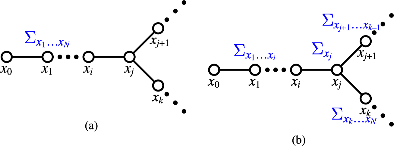
Consider Figure 29.7, showing a section of a general network with pairwise potentials. There is a network of \(N+1\) nodes, numbered \(0\) through \(N\) and we will marginalize over nodes \(x_1 \ldots x_N\). Figure 29.7 (a) shows the marginalization equation for a network of variables with discrete states. (For continuous variables, integrals replace the summations). If we assume the nodes form a tree, we can distribute the marginalization sum past nodes for which the sum is a constant value to obtain the sums depicted in Figure 29.7 (b).
We define a belief propagation message: A message \(m_{ij}\), from node \(i\) to node \(j\), is the sum of the probability over all states of all nodes in the subtree that leaves node \(i\) and does not include node \(j\).
Referring to Figure 29.7 (a), shows the desired marginalization sum over a network of pairwise cliques. We can pass the summations over node states through nodes that are constant over those summations, arriving at the factorization shown in Figure 29.7 (b). Remembering that the message from node \(j\) to node \(i\) is the sum over the tree leaving node \(j\), we can then read-off the recursive belief propagation message update rule by marginalizing over the state probabilities at node \(j\) in Figure 29.7. As illustrated in Figure 29.7, messages \(m_{j+1,j}\) and \(m_{kj}\) correspond to partial sums over nodes indicated in the graph: \(m_{j+1,j} = \sum_{x_{j+1} \ldots x_{k-1}}\) and \(m_{kj} = \sum_{x_k \ldots x_N}\). Marginalization over the states of all nodes leaving node \(j\), not including node \(i\), leads to equation (Equation 29.7), the belief propagation message passing rule.
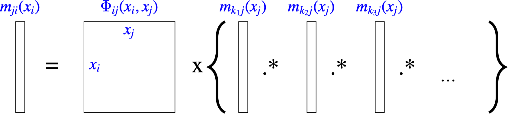
To compute the message from node \(j\) to node \(i\):
Multiply together all messages (independent probabilities) coming in to node \(j\), except for the message from node \(i\) back to node \(j\),
Multiply by the pairwise compatibility function \(\psi_{ij}(x_i, x_j)\) (also independent of the other multiplicands).
Marginalize over the variable \(x_j\).
These steps are summarized in this equation to compute the message from node \(j\) to node \(i\):
\[m_{j i}\left(x_i\right)=\sum_{x_j} \psi_{i j}\left(x_i, x_j\right) \prod_{k \in \eta(j) \backslash i} m_{k j}\left(x_j\right) \tag{29.7}\]
where \(\eta(j) \backslash i\) means “the neighbors of node \(j\) except for node \(i\).” Figure 29.8 shows this equation in a graphical form. Any local potential functions \(\phi_{j}(x_j)\) are treated as an additional message into node \(j\), that is, \(m_{0j}(x_j) = \phi_{j}(x_j)\). For the case of continuous variables, the sum over the states of \(x_j\) in equation (Equation 29.7) is replaced by an integral over the domain of \(x_j\).
As mentioned previously, BP messages are partial sums in the marginalization calculation. The arguments of messages are always the state of the node that the message is going to. (BP follows the “nosey neighbor rule” (from Brendan Frey, Univ. Toronto): Every node is a house in some neighborhood. Your nosey neighbor says to you, “Given what I’ve seen myself and everything I’ve heard from my neighbors, here’s what I think is going on inside your house.” (That metaphor especially makes sense if one has teenaged children.)
29.6.2 Marginal Probability
The marginal probability at a node \(i\), equation (Equation 29.3), is the sum over the joint probabilities of all states except those of \(x_i\). Because we assume the network has no loops, the conditional independence structure assures us that marginal probability at a node \(i\) is the product of the sum of all states of all nodes in each subtree connected to node \(i\): Conditioned on node \(i\), the probabilities within each subtree are independent. Thus the marginal probability at node \(i\) is the product of all the incoming messages: \[p_{i}(x_i) = \prod_{j\in \eta(i)} m_{ji}(x_i) \tag{29.8}\] (We include the local clique potential at node \(i\), \(\psi_i(x_i)\), as one of the messages in the product of all messages into node \(i\)).
29.6.3 Message Update Sequence
To find all the messages, how do we invoke the recursive BP update rule, equation (Equation 29.7)? We can apply equation (Equation 29.7) whenever all the incoming messages in the BP update rule are defined. If there are no incoming messages to a node, then its outgoing message is well-defined in the update rule. This lets us start the recursive algorithm.
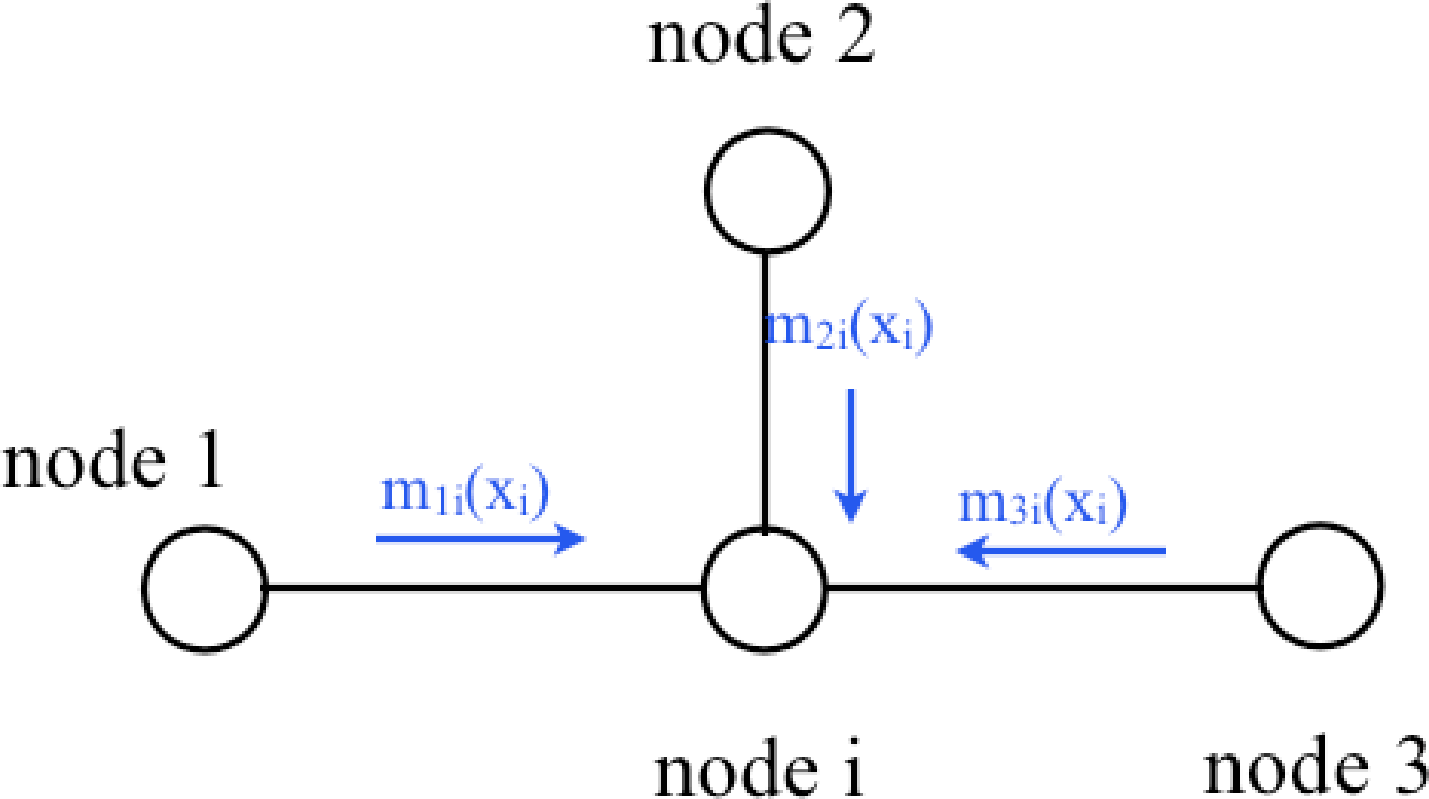
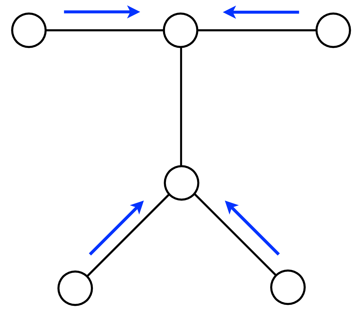
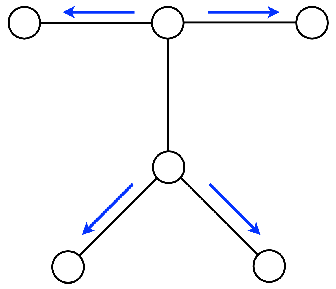
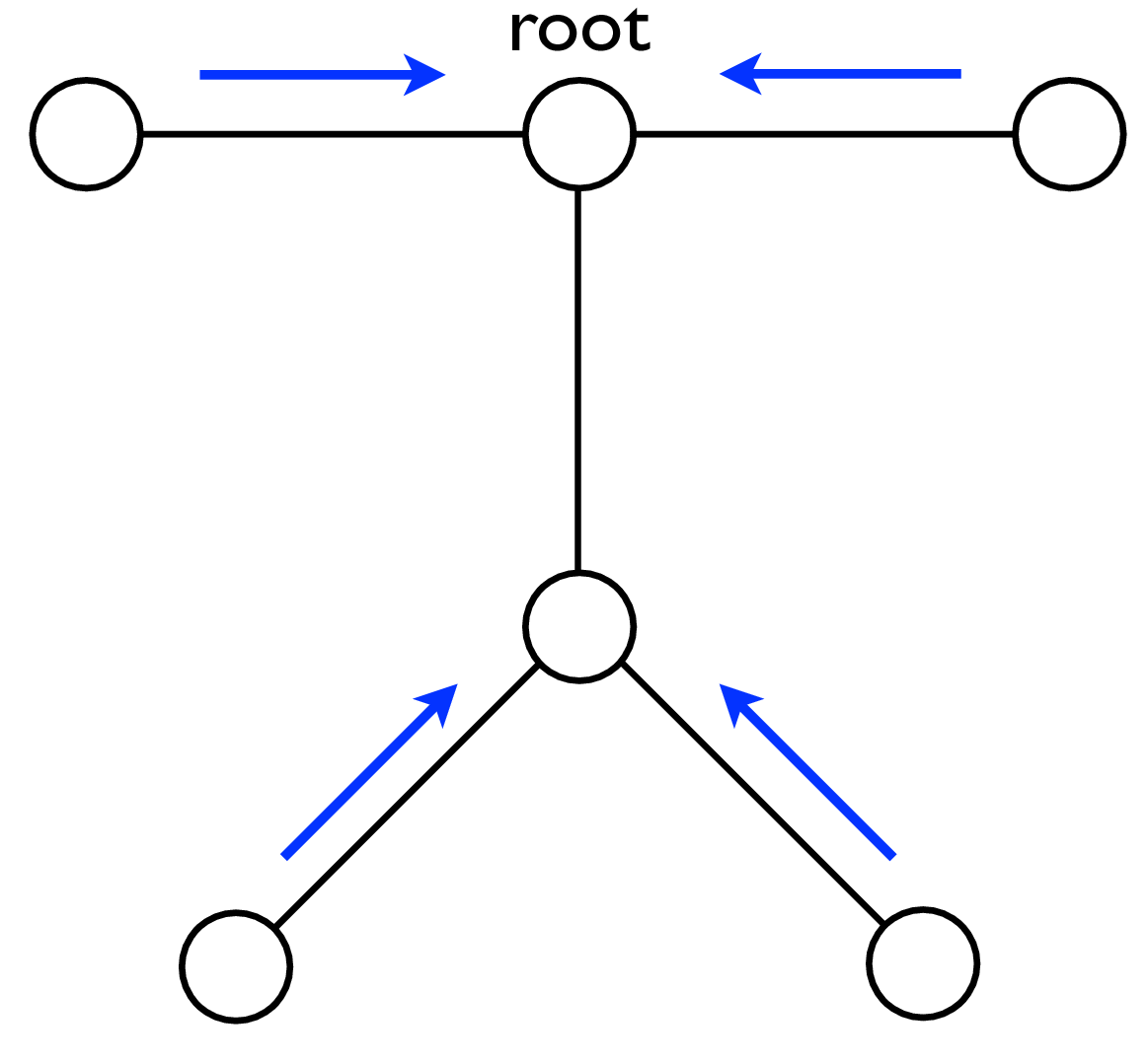
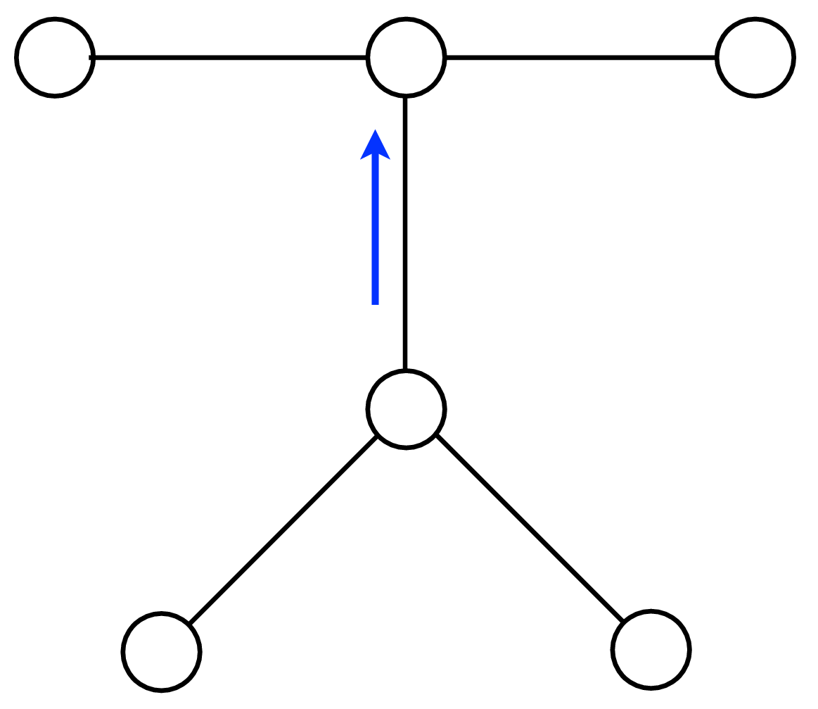
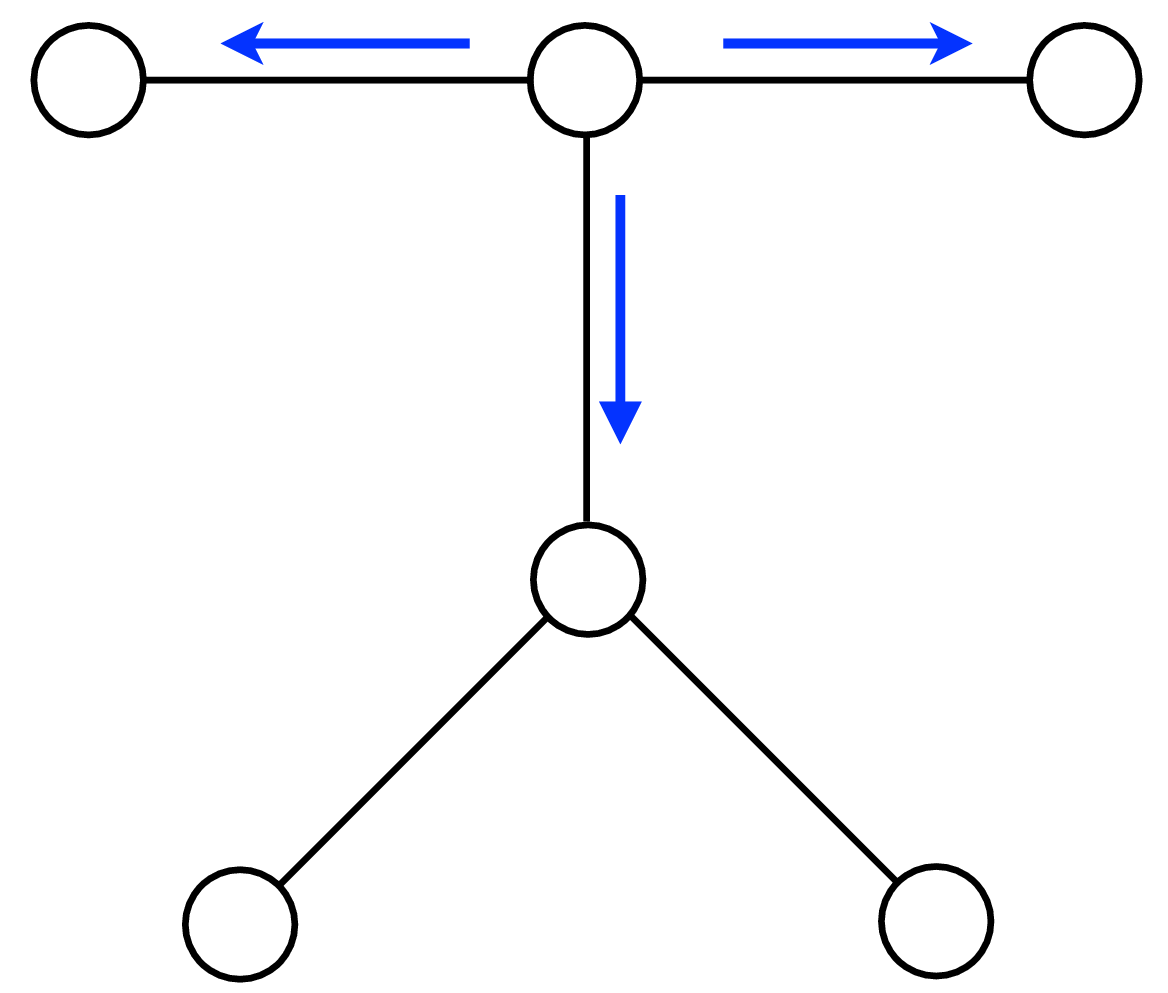
A node can send a message whenever all the incoming messages it needs have been computed. We can compute the outgoing messages from leaf nodes in the graphical model tree, since they have no incoming messages other than from the node to which they are sending a message, which doesn’t enter in the outgoing message computation. Two natural message passing protocols are consistent with that rule: depth-first update, and parallel update. In depth-first update, one node is arbitrarily picked as the root. Messages are then passed from the leaves of the tree (leaves, relative to that root node) up to the root, then back down to the leaves. In parallel update, at each turn, every node sends every outgoing message for which it has received all the necessary incoming messages. Figure 29.10 depicts the flow of messages for the parallel, synchronous update scheme and Figure 29.11 shows the flow for the same network, but with a depth-first update schedule.
Note that when computing marginals at many nodes, we reuse messages with the BP algorithm. A single message-passing sweep through all the nodes lets us calculate the marginal at any node (using the depth-first update rules to calculate the marginal at the root node). A second sweep from the root node back to all the leaf nodes calculates all the messages needed to find the marginal probability at every node. It takes only twice the number of computations to calculate the incoming messages to every node, and thus the marginal probabilities everywhere, as it does to calculate the incoming messages for the marginal probability at a single node.
29.6.4 Example Belief Propagation Application: Stereo
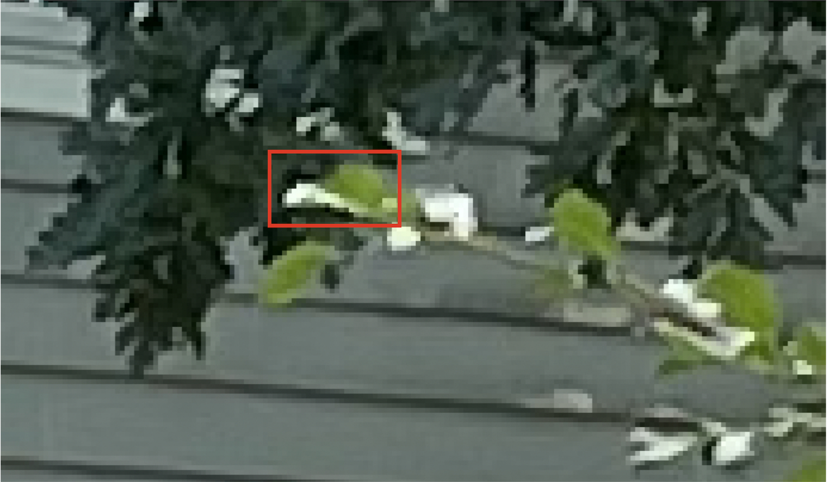
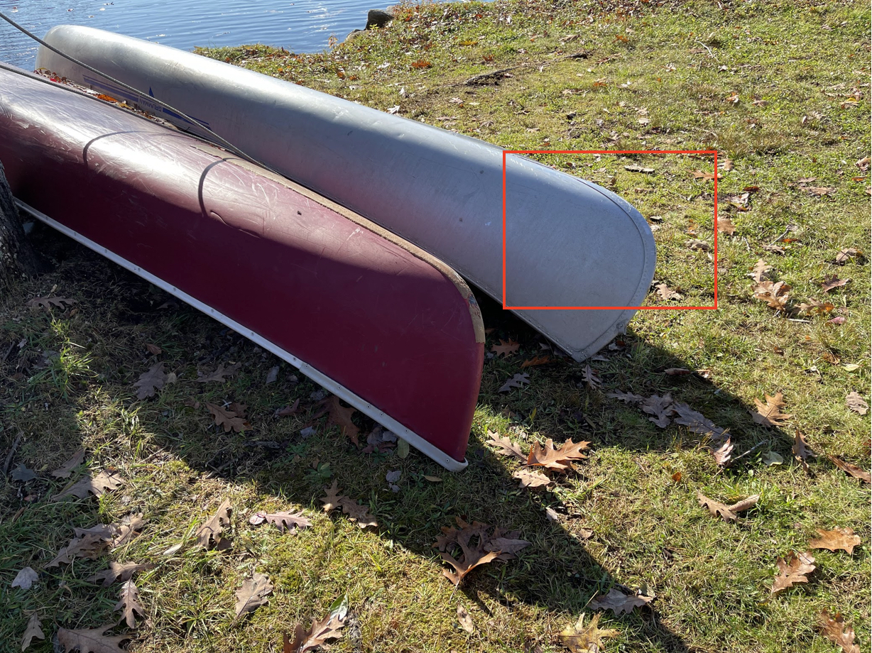
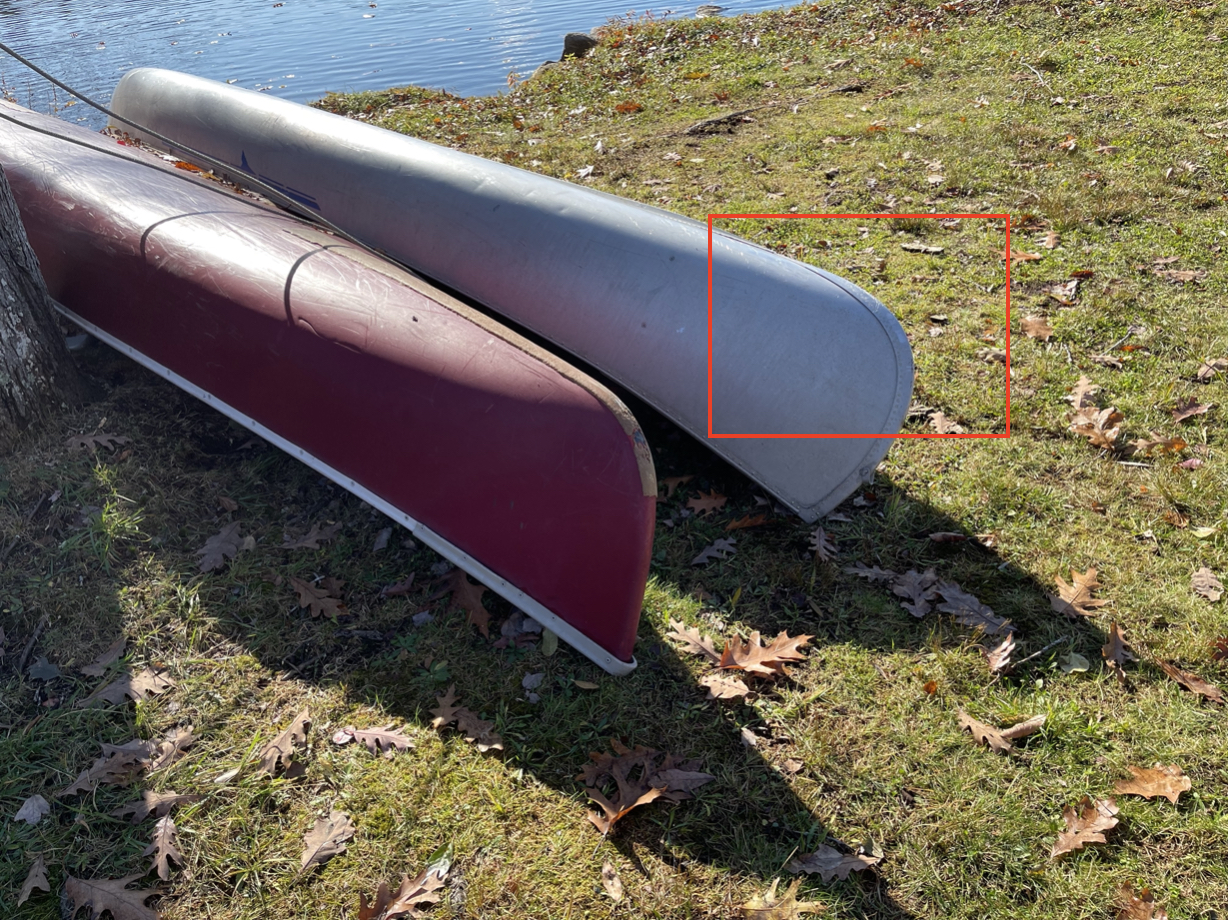
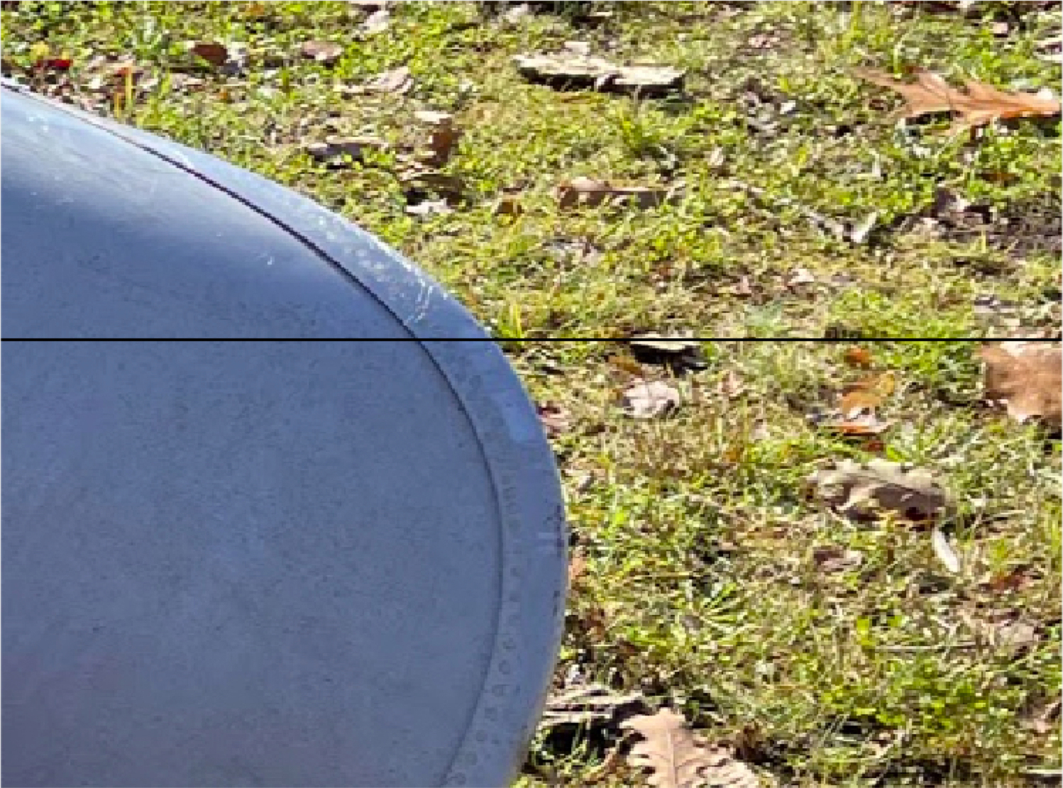
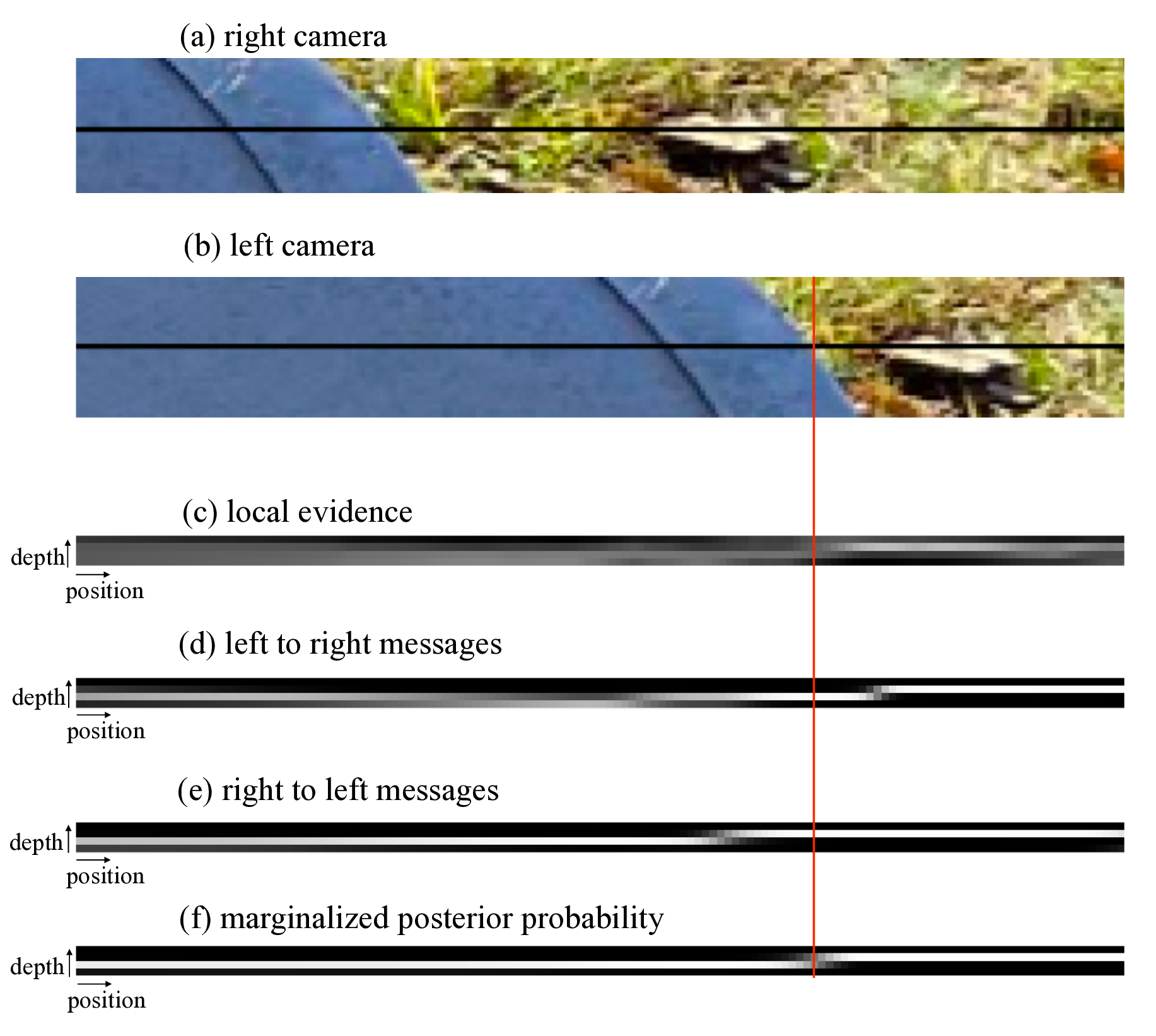
Assume that we want to compute the depth from a stereo image pair, such as the pair shown in Figure 29.12(a and b) and with their insets marked with the red rectangles, shown in Figure 29.12(c and d). Assume that the two images have been rectified, as described in Chapter 40, and consider the common scanline, marked in Figure 29.12(c and d) with a black horizontal line. The luminance intensities of each scanline are plotted in Figure 29.12(e and f). Most computer vision stereo algorithms [6] examine multiple scanlines to compute the depth at every pixel, but to illustrate a simple example of belief propagation in vision, we will consider the stereo vision problem while considering only one scanline pair at a time.

The graphical model that describes this stereo depth reconstruction for a single scanline is shown in Figure 29.13.
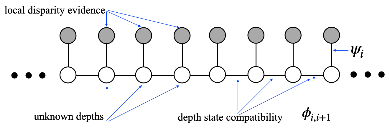
Each unfilled circle in the graphical model (Figure 29.13) represents the unknown depth of each pixel in the scan line of one of the stereo images, in this example, the left camera image in Figure 29.12 (c). The open circles mean that the depth of each pixels is an unobserved variable. Often, we represent the depth as the disparity between the left and right camera images, see Chapter 40.
The intensity values of the left and right camera scan lines can be used to compute the local evidence for the disparity offset, \(d[i, j]\), of each right camera pixel corresponding to the left image pixel at each right camera position, \([i,j]\). For this example, we assume that each right camera pixel value, \(\boldsymbol\ell_r\) is that of a corresponding left camera value, \(\boldsymbol\ell_l\), but with independent, identically distributed (IID) Gaussian random noise added. This leads to a simple formula for the local evidence, \(\psi_i\), for the given depth value of any pixel,
\[\psi_i = p(d[i,j] \bigm | \boldsymbol\ell_r, \boldsymbol\ell_l) = k \exp{\left( -\sum_{i=-10}^{i=10} \frac{(\boldsymbol\ell_r[i,j] - \boldsymbol\ell_l[i - d[i, j], j])^2}{2 \sigma^2} \right)}\]
For simplicity in this example, we discretize the disparity offsets into four different bins, each 45 disparity pixels wide. We sum the local disparity evidence within each depth bin, then normalize the evidence at each position to maintain a probability distribution. The resulting local evidence matrix, for each of the four depth states, at each left camera spatial position, is displayed in Figure 29.14 (c). The intensities in each column in the third-row image add up to one.
The prior probability of any configuration of pixel disparity states is described by setting the compatibility matrices, \(\mathbf{\phi}[s_i, s_{i+1}]\) of the Markov chain of Figure 29.13. For this example, we use a compatibility matrix referred to as the Potts Model [7]:
\[\mathbf{\phi}[s_i, s_{i+1}] = \begin{cases} 1, & \text{if}\ s_i = s_{i+1} \\ \delta, & \text{otherwise} \end{cases}\]
For this example, we used \(\delta = 0.001\)
We then ran BP (Equation 29.7) in a depth-first update schedule. For this network, that involves two linear sweeps over all the nodes of the chain, first from left to right, then from right to left. Starting from the left-most node, we updated the rightward messages one node at a time, in a rightward sweep; then, starting from the right-most node, updated all the leftward messages one node at a time, in a leftward sweep. The results are in Figure 29.14 (d and e), respectively.
Once all the messages were computed, we used equation (Equation 29.8) to find the posterior marginal probability at each node. That involves, at each position, multiplying together all the incoming messages, including the local evidence. Thus, the values shown in Figure 29.14 (f) are the product, at each position, of Figure 29.14 (c, d and e). Note that for this scanline, in this image pair, there is a depth discontinuity at location of the red vertical mark in Figure 29.14, namely the canoe is closer to the camera than the ground beyond the canoe that appears to the right of the canoe. The local evidence for depth disparity, Figure 29.14 (c), is rather noisy, but the marginal posterior probability, after aggregating evidence along the scanline, accurately finds the depth discontinuity at the canoe boundary.
29.7 Loopy Belief Propagation
The BP message update rules only work to give the exact marginals when the topology of the network is that of a tree or a chain. In general, one can show that exact computation of marginal probabilities for graphs with loops depends on a graph-theoretic quantity known as the treewidth of the graph [4]. For many graphical models of interest in vision, such as 2D Markov random fields related to images, these quantities can be intractably large. Message update rules are described locally, and one might imagine that it is a useful local operation to perform, even without the global guarantees of ordinary BP. It turns out that is true. Here is the algorithm, also know as loopy belief propagation algorithm:
Convert graph to pairwise potentials.
Initialize all messages to all ones, or to random values between 0 and 1.
Run the belief propagation update rules of Section 29.6.1 until convergence.
One can show that, in networks with loops, fixed points of the belief propagation algorithm (message configurations where the messages don’t change with a message update) correspond to minima of a well-known approximation from the statistical physics community known as the Bethe free energy [8]. In practice, the solutions found by the loopy belief propagation algorithm can be quite good [9].
Instead of summing over the states of other nodes, we are sometimes interested in finding the \(\mathbf{x}\) that maximizes the joint probability. The argmax operator passes through constant variables just as the summation sign did. This leads to an alternate version of the BP algorithm, equation (Equation 29.7), with the summation (of multiplying the vector message products by the node compatibility matrix) replaced with argmax. This is called the max-product version of belief propagation, and it computes an MAP estimate of the hidden states. Improvements have been developed over loopy belief propagation for the case of MAP estimation; see, for example, tree-reweighted belief propagation [10] and graph cuts [11].
29.7.1 Numerical Example of Belief Propagation
Here we work though a numerical example of belief propagation. To make the arithmetic easy, we’ll solve for the marginal probabilities in the graphical model of two-state (0 and 1) random variables shown in Figure 29.15.

That graphical model has three hidden variables, and one variable observed to be in state 0. The compatibility matrices are given in the arrays below (for which the state indices are 0, then 1, reading from left to right and top to bottom): \[\psi_{12}(x_1, x_2) = \begin{bmatrix} 1.0 & 0.9 \\ 0.9 & 1.0 \end{bmatrix}\] \[\psi_{23}(x_2, x_3) = \begin{bmatrix} 0.1 & 1.0 \\ 1.0 & 0.1 \end{bmatrix}\] \[\psi_{42}(x_2, y_2) = \begin{bmatrix} 1.0 & 0.1 \\ 0.1 & 1.0 \end{bmatrix}\] Note that in defining these potential functions, we haven’t taken care to normalize the joint probability, so we’ll need to normalize each marginal probability at the end (remember \(p(x_1, x_2, x_3, y_2) = \psi_{42}(x_2, y_2) \psi_{23}(x_2, x_3) \psi_{12}(x_1, x_2)\), which should sum to 1 after summing over all states).
For this simple toy example, we can tell what results to expect by inspection, then verify that BP is doing the right thing. Node \(x_2\) wants very much to look like \(y_2=0\), because \(\psi_{42}(x_2, y_2)\) contributes a large valued to the posterior probability when \(x_2 = y_2 = 1\) or when \(x_2 = y_2 = 0\). From \(\psi_{12}(x_1, x_2)\) we see that \(x_1\) has a very mild preference to look like \(x_2\). So we expect the marginal probability at node \(x_2\) will be heavily biased toward \(x_2=0\), and that node \(x_1\) will have a mild preference for state 0. \(\psi_{23}(x_2, x_3)\) encourages \(x_3\) to be the opposite of \(x_2\), so it will be biased toward the state \(x_3=1\).
Let’s see what belief propagation gives. We’ll follow the parallel, synchronous update scheme for calculating all the messages. The leaf nodes can send messages along their edges without waiting for any messages to be updated. For the message from node 1, we have
\[\begin{aligned} m_{12}(x_2) &= \sum_{x_1} \psi_{12} (x_1, x_2) \nonumber \\ &= \begin{bmatrix} 1.0 & 0.9 \\ 0.9 & 1.0 \end{bmatrix} \begin{bmatrix} 1 \\ 1 \end{bmatrix} = \begin{bmatrix} 1.9 \\ 1.9 \end{bmatrix} = k_1 \begin{bmatrix} 1 \\ 1 \end{bmatrix} \end{aligned}\]
For numerical stability, we typically normalize the computed messages in equation (Equation 29.7) so the entries sum to 1, or so their maximum entry is 1, then remember to renormalize the final marginal probabilities to sum to 1. Here, we will normalize the messages for simplicity, absorbing the normalization into constants, \(k_i\).
The message from node 3 to node 2 is \[\begin{aligned} m_{32}(x_2) &= \sum_{x_3} \psi_{32} (x_2, x_3) \nonumber \\ &= \begin{bmatrix} 0.1 & 1.0 \\ 1.0 & 0.1 \end{bmatrix} \begin{bmatrix} 1 \\ 1 \end{bmatrix} = \begin{bmatrix} 1.1 \\ 1.1 \end{bmatrix} = k_2 \begin{bmatrix} 1 \\ 1 \end{bmatrix} \end{aligned}\]
We have a nontrivial message from observed node \(y_2\) (node 4) to the hidden variable \(x_2\):
\[\begin{aligned} m_{42}(x_2) &= \sum_{x_4} \psi_{42} (x_2, y_2) \nonumber \\ &= \begin{bmatrix} 1.0 & 0.1 \\ 0.1 & 1.0 \end{bmatrix} \begin{bmatrix} 1 \\ 0 \end{bmatrix} = \begin{bmatrix} 1.0 \\ 0.1 \end{bmatrix} \end{aligned}\] where \(y_2\) has been fixed to \(y_2 = 0\), thus restricting \(\psi_{42} (x_2, y_2)\) to just the first column.
Now we just have two messages left to compute before we have all messages computed (and therefore all node marginals computed from simple combinations of those messages). The message from node 2 to node 1 uses the messages from nodes 4 to 2 and 3 to 2: \[\begin{aligned} m_{21}(x_1) &= \sum_{x_2} \psi_{12} (x_1, x_2) m_{42}(x_2) m_{32}(x_2) \nonumber \\ &= \begin{bmatrix} 1.0 & 0.9 \\ 0.9 & 1.0 \end{bmatrix} \left( \begin{bmatrix} 1.0 \\ 0.1 \end{bmatrix} \odot \begin{bmatrix} 1 \\ 1 \end{bmatrix} \right) = \begin{bmatrix} 1.09 \\ 1.0 \end{bmatrix} \end{aligned}\]
The final message is that from node 2 to node 3 (since \(y_2\) is observed, we don’t need to compute the message from node 2 to node 4). That message is: \[\begin{aligned} m_{23}(x_3) &= \sum_{x_2} \psi_{23} (x_2, x_3) m_{42}(x_2) m_{12}(x_2) \nonumber \\ &= \begin{bmatrix} 0.1 & 1.0 \\ 1.0 & 0.1 \end{bmatrix} \left( \begin{bmatrix} 1.0 \\ 0.1 \end{bmatrix} \odot \begin{bmatrix} 1 \\ 1 \end{bmatrix} \right) = \begin{bmatrix} 0.2 \\ 1.01 \end{bmatrix} \end{aligned}\]
Now that we’ve computed all the messages, let’s look at the marginals of the three hidden nodes. The product of all the messages arriving at node 1 is just the one message, \(m_{21}(x_1)\), so we have (introducing constant \(k_3\) to normalize the product of messages to be a probability distribution) \[p_1(x_1) = k m_{21}(x_1) = \frac{1}{2.09} \begin{bmatrix} 1.09 \\ 1.0 \end{bmatrix}\] As we knew it should, node 1 shows a slight preference for state 0.
The marginal at node 2 is proportional to the product of three messages. Two of those are trivial messages, but we’ll show them all for completeness: \[\begin{aligned} p_2(x_2) &= k_4 m_{12}(x_2) m_{42}(x_2) m_{32}(x_2) \\ &= k_4 \begin{bmatrix} 1 \\ 1 \end{bmatrix} \odot \begin{bmatrix} 1.0 \\ 0.1 \end{bmatrix} \odot \begin{bmatrix} 1 \\ 1 \end{bmatrix} = \frac{1}{1.1} \begin{bmatrix} 1.0 \\ 0.1 \end{bmatrix} \end{aligned}\] As expected, belief propagation reveals a strong bias for node 2 being in state 0.
Finally, for the marginal probability at node 3, we have \[p_3(x_3) = k_5 m_{23}(x_3) = \frac{1}{1.21} \begin{bmatrix} 0.2 \\ 1.01 \end{bmatrix}\]
As predicted, this variable is biased toward being in state 1.
By running belief propagation within this tree, we have computed the exact marginal probabilities at each node, reusing the intermediate sums across different marginalizations, and exploiting the structure of the joint probability to perform the computation efficiently. If nothing were known about the joint probability structure, the marginalization cost would grow exponentially with the number of nodes in the network. But if the graph structure corresponding to the joint probability is known to be a chain or a tree, then the marginalization cost only grows linearly with the number of nodes, and is quadratic in the node state dimensions. The belief propagation algorithm enables inference in many large-scale problems.
29.8 Relationship of Probabilistic Graphical Models to Neural Networks
The probabilistic graphical models (PGMs) we studied in this chapter and neural networks (NNs) share some characteristics, but are quite different. Both share a graph structure, with nodes and edges, but the nodes and edges mean different things in each case. Below is a brief summary of the differences:
Nodes: The nodes of a NN diagram typically represent a real-valued scalar activations. The nodes of a PGM represent a random variable, real or discrete-valued, and scalars or vectors.
Edges: Edges in PGMs determine statistical dependencies. Edges in NNs determine which are involved in a linear summation to the next layer.
Computation: The big difference between PGMs and NNs lies in what they calculate. PGMs represent factorized probability distributions and pass messages that allow for the computation of probabilities, for example, the marginal probability at a node. In contrast, NNs compute results that minimize some expected loss or an energy function [12], [13]. That different goal, that is, minimizing an expected loss rather than calculating a probability, allows for more general computations by a neural network at the cost of output that may be less modular or less interpretable because they are not probabilities.
Both PGMs and NNs can have nodes organized into grid-like structures but also more generally in arbitrary graphs; see, for example, [14], [15].
29.9 Concluding Remarks
Probabilistic graphical models provide a modular representation for complex joint probability distributions. Nodes can represent pixels, scenes, objects, or object parts, while the edges describe the conditional independence structure. For tree-like graphs, belief propagation delivers optimal inference. In general graphs with loops, it can give a reasonable approximation.