33 Generative Modeling Meets Representation Learning
33.1 Introduction
This chapter is about models that unite the ideas of both generative modeling and representation learning. These models learn mappings both to and from data.
The intuition is that generative models map a simple base distribution (i.e., noise) to data, whereas representation learning maps data to simple underlying representations (embeddings). These two problems are, essentially, inverses of each other. Many algorithms explicitly treat them as inverse problems, where solving the problem in one direction can inform the solution in the other direction.
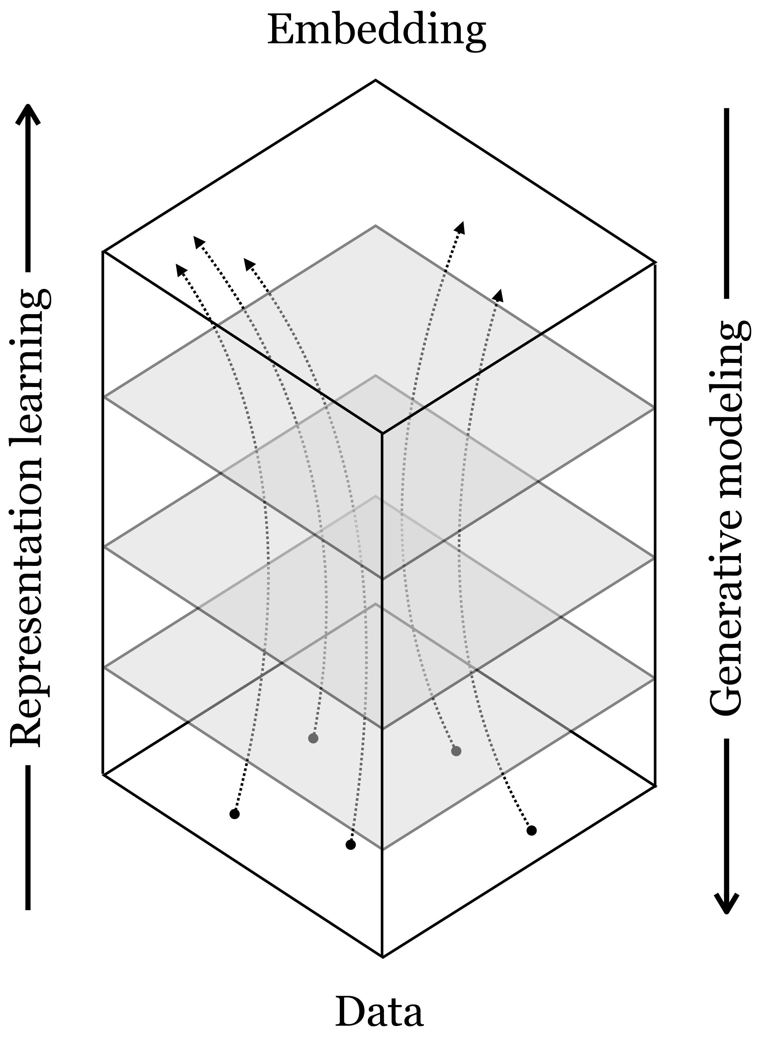
In Chapter 12, we described neural nets as being a sequence of mappings from raw data to ever more abstracted representations, layer by layer. This perspective puts representation learning in the spotlight: deep learning is just representation learning! Let us now point out an alternative perspective: in backward order, deep nets are mappings from abstracted representations to ever more concrete representations of the data, layer by layer. This backward ordering is the direction in which deep generative networks work. This perspective puts the spotlight on generative modeling: deep learning is just generative modeling! Indeed both modeling directions are valid, and the full picture looks like this (Figure 33.1):
Moving backward through a net is also what backpropagation does, but it computes a different function: backpropagation computes the gradient \(\nabla f\) whereas here we focus on the inverse \(f^{-1}\).
33.2 Latent Variables as Representations
In Chapter 32, we introduced generative models with latent variables \(\mathbf{z}\). In that context, the role of the latent variable was to specify all unobserved factors that might affect the output of a model. For example, if the model predicts the color of a black and white photo, it is a mapping \(g: \mathbf{x}, \mathbf{z} \rightarrow \mathbf{y}\), with \(\mathbf{x}\) being the black and white input, \(\mathbf{y}\) being the color output and \(\mathbf{z}\) being any other information that needs to be known in order to make the mapping completely deterministic; for example, the color of a t-shirt which cannot be inferred solely from the black and white input. In the extreme case of unconditional generative models, all properties of the generated images are controlled by the latent variables.
What we did not mention in Chapter 32, but will focus on now, is that latent variables are representations of the data. In the case of an unconditional generative model, the latent variables are a complete representation of the data: all information in the data is represented in the latent variables.
Given this connection, this chapter will ask the following question: Are latent variables good representations of the data? And can they be combined with other representation learning algorithms?
33.3 Technical Setting
We will consider random variables \(\mathbf{z}\) and \(\mathbf{x}\) related as follows, with \(g\) being deterministic generator (i.e., decoder) and \(f\) being a deterministic encoder:
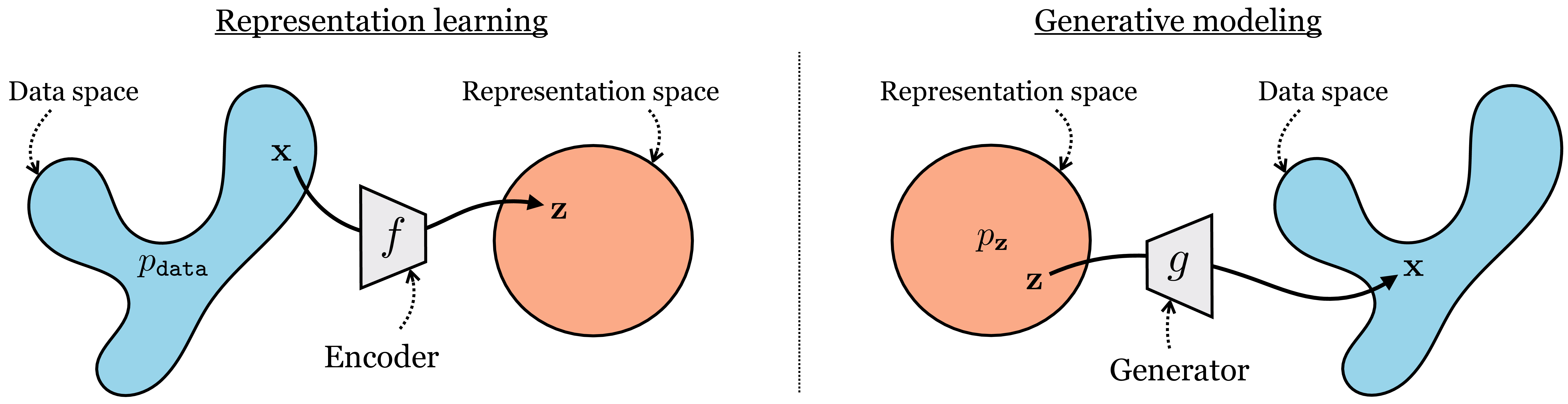
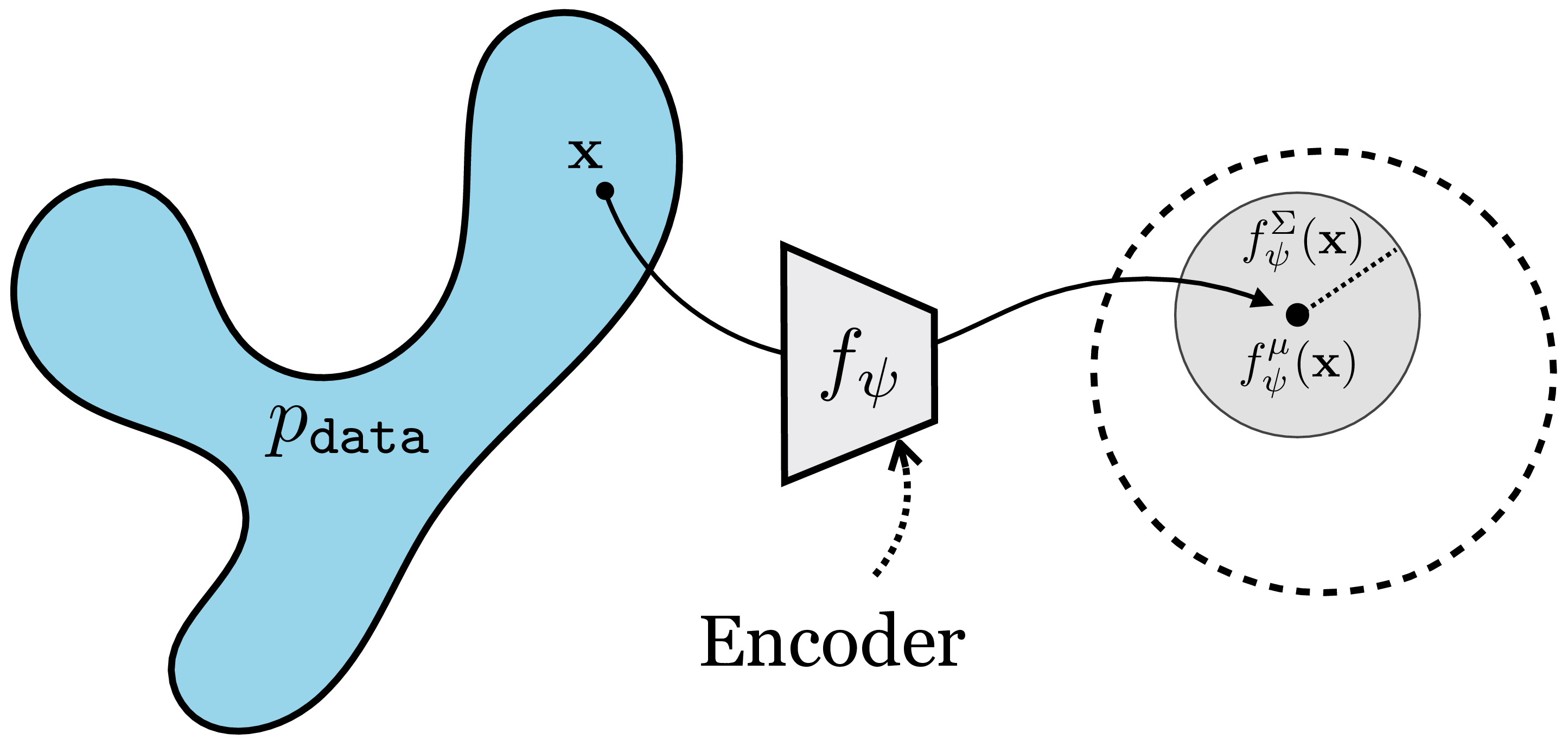
\[\begin{aligned} &\mathbf{x} \sim p_{\texttt{data}} &\mathbf{z} \sim p_{\mathbf{z}} \\ &\hat{\mathbf{z}} = f(\mathbf{x}) &\hat{\mathbf{x}} = g(\mathbf{z}) \end{aligned}\] where \(f\) and \(g\) will be trained so that \(g \approx f^{-1}\), which means that \(\hat{\mathbf{x}} \approx \mathbf{x}\) and \(\hat{\mathbf{z}} \approx \mathbf{z}\). In Figure 30.1, we sketched how representation learning maps from a data domain to a simple embedding space. We can now put that diagram side by side with the equivalent diagram for generative modeling. Notice again how they are just the same thing in opposite directions (Figure 33.2):
The critical thing in most generative models, which is not necessarily true for representation learning models, is that we assume we know the distribution \(p_{\mathbf{z}}\), and typically it has a simple form such as a unit Gaussian. Knowing this distribution allows us to sample from it and then generate images via \(g\).
One of the most important quantities we will measure is the data log likelihood function \(L(\{\mathbf{x}\}_{i=1}^N, \theta)\), which measures the log likelihood of the data under the model \(p_{\theta}\): \[\begin{aligned} L(\{\mathbf{x}^{(i)}\}_{i=1}^N, \theta) = \sum_{i=1}^N \log p_{\theta}(\mathbf{x}^{(i)}) \end{aligned}\] Many methods use a max likelihood objective, optimizing \(L\) with respect to \(\theta\). To compute the likelihood function, we need to compute \(p_{\theta}(\mathbf{x})\).
One way to express this function is as the marginal likelihood of \(\mathbf{x}\), marginalizing over all unobserved latent variables \(\mathbf{z}\): \[\begin{aligned} p_{\theta}(\mathbf{x}) = \int_{\mathbf{z}} p_{\theta}(\mathbf{x} \bigm | \mathbf{z})p_{\mathbf{z}}(\mathbf{z})d\mathbf{z} \end{aligned} \tag{33.1}\]
The advantage of expressing \(p_{\theta}(\mathbf{x})\) in this way is that, assuming we know \(p_{\mathbf{z}}\), the rest of the modeling problem is reduced to learning the conditional distribution \(p_{\theta}(X \bigm | \mathbf{z})\), which itself can be straightforwardly modeled using \(g\). For example, we could model \(p_{\theta}(X \bigm | \mathbf{z}) = \mathcal{N}(\mu = g(\mathbf{z}), \sigma = \mathbf{1})\), that is, just place a unit Gaussian distribution over \(X\) centered on \(g(\mathbf{z})\).
The integral in Equation 33.1 is expensive so most generative models either sidestep the need to explicitly calculate it, or approximate it. We will examine one such strategy next.
33.4 Variational Autoencoders
In the next sections we will examine the variational autoencoder (VAE) [1], [2], which is a model that turns an autoencoder into a generative model that can synthesize data.
33.4.1 The Decoder of an Autoencoder is a Data Generator
In Chapter 30 we learned about autoencoders. These are models that learn an embedding that can be decoded to reconstruct the input data. You may already have noticed that the decoder of an autoencoder looks just like a generator. It is a mapping from a representation of the data, \(\mathbf{z}\), back to the data itself, \(\mathbf{x}\). Given a \(\mathbf{z}\), we can synthesize an image by passing it through the decoder of the autoencoder (Figure 33.3):
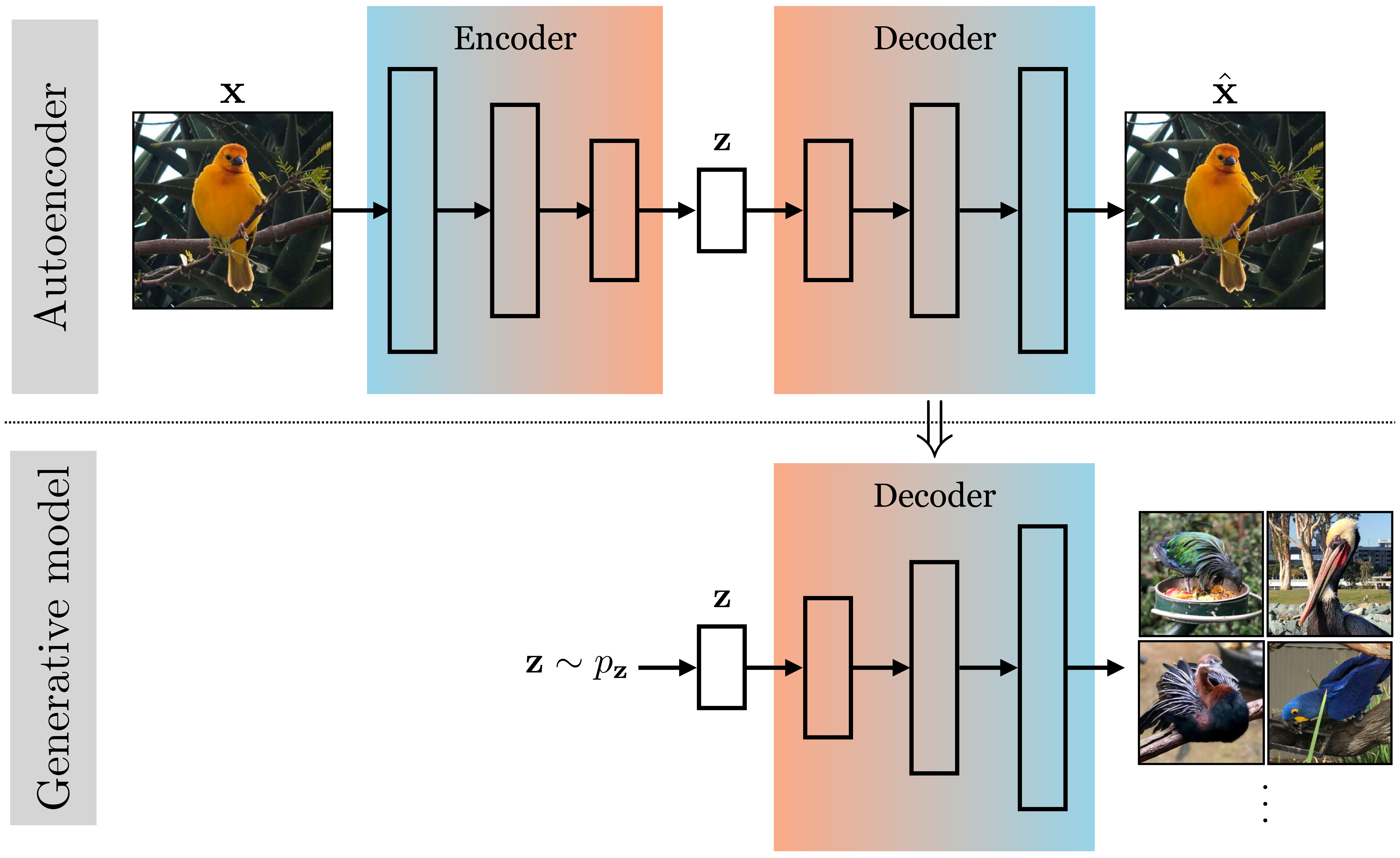
But how do we get this \(\mathbf{z}\)? One goal of generative modeling is to be able to make up random images from scratch. So we need a distribution from which we can sample different \(\mathbf{z}\) from scratch, that is, we need \(p_{\mathbf{z}}\). An autoencoder doesn’t directly give us this. You might ask, what if, after training an autoencoder, you just sample a random \(\mathbf{z}\), say from a unit Gaussian, and feed it through the decoder? The problem is that this sample might be very different from what the decoder was trained on, and it therefore might not map to a natural looking image. For example, maybe the encoder has learned to map all images to embeddings far from the origin; then a unit Gaussian \(\mathbf{z}\) would be far out of distribution and the decoder’s behavior could be arbitrary for this out-of-distribution input.
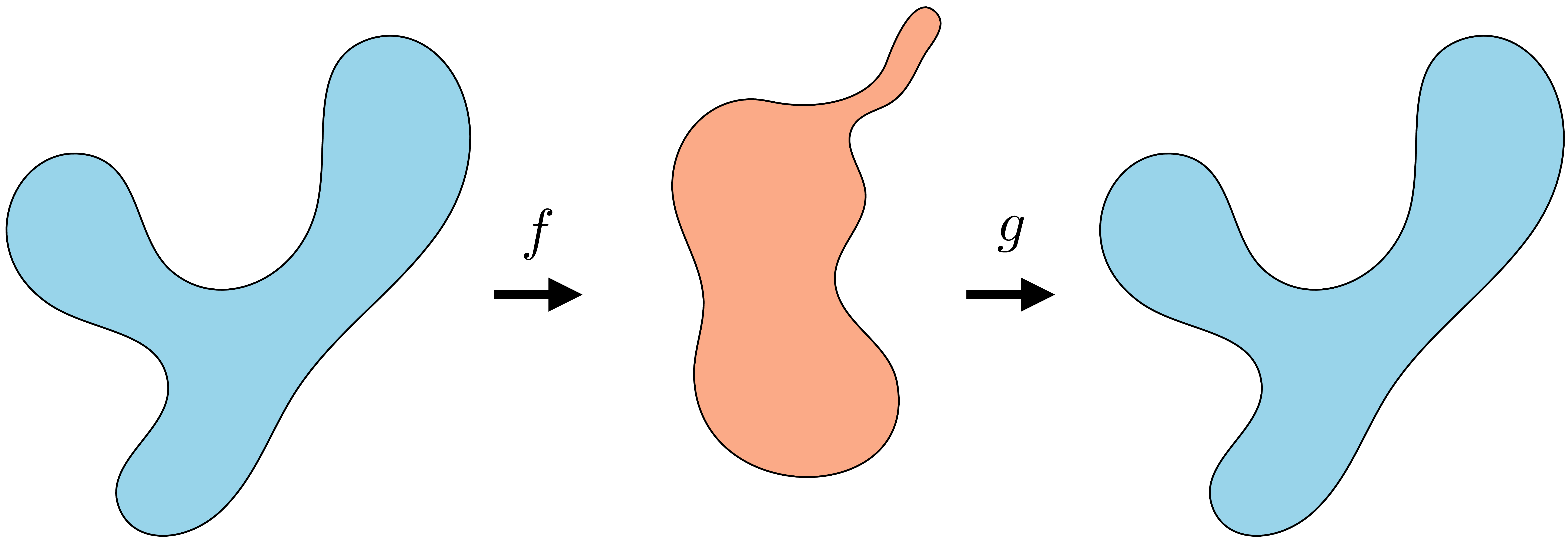
In general, the embedding space of an autoencoder might be just as complicated to model as the data space we started with, as indicated in Figure 33.4:
Variational autoencoders VAEs are a way to turn an autoencoder into a proper generative model, which can be sampled from and which maximizes data likelihood under a formal probabilistic model. The trick is very simple: just take a vanilla autoencoder and (1) regularize the latent distribution to squish it into a Gaussian (or some other base distribution), (2) add noise to the output of the encoder. In code, it can be as simple as a two line change!
Okay, but seeing why this is the right and proper thing to do requires quite a bit of math. We will derive it now, using a different approach than in most texts. We think this approach makes it easier to intuit what is going on. See [2] for the more standard derivation.
33.4.2 The VAE Hypothesis Space
VAEs are max likelihood generative models, which maximize the likelihood function \(L\) in Equation 33.1. What distinguishes them from other max likelihood models is their particular hypothesis space and optimization algorithm. We will first describe the hypothesis space.
Remember the Gaussian generative model from Chapter 32 (i.e., fitting a Gaussian to data)? We stated that this model is too simple for most purposes, but can form the basis for more flexible density models, which work by combining a lot of simple distributions. We gave one example in Chapter 32: autoregressive models, which model a complicated distribution as a product over many simple conditional distributions. VAEs follow a slightly different strategy: they model complicated distributions as sums of simple distributions.
Mixture models are probability models of the form \(P(\mathbf{x}) = \sum_i w_ip_i(\mathbf{x})\).
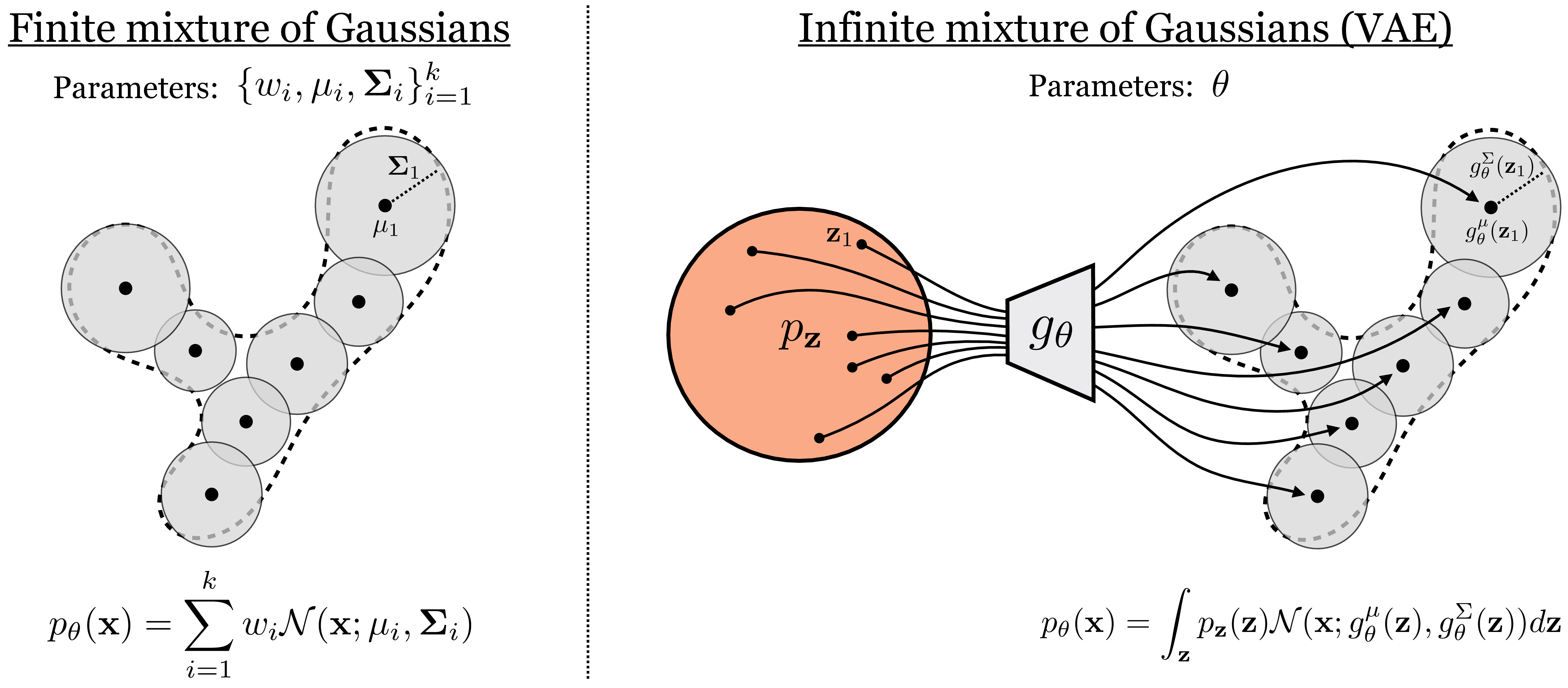
In particular, VAEs are mixture models, and the most common kind of VAE is a mixture of Gaussians. The mixture of Gaussians model is in fact classical model that represents a density as a weighted sum of Gaussian distributions:
\[\begin{aligned} p_{\theta}(\mathbf{x}) = \sum_{i=1}^k w_i \mathcal{N}(\mathbf{x}; \mathbf{\mu}_i, \mathbf{\Sigma}_i) \quad\quad \triangleleft \quad\text{mixture of Gaussians} \end{aligned}\] where the parameters are \(\theta = \{\mathbf{\mu}_i, \mathbf{\Sigma}_i\}_{i=1}^k\), that is, the mean and variance of all Gaussians in the mixture. Unlike classical Gaussian mixture models, VAEs use an infinite mixture of Gaussians, that is, \(k \rightarrow \infty\).
But wait, how can we parameterize an infinite mixture? We can’t learn an infinite set of means and variances. The trick we will use is to make the mean and variance be functions of an underlying continuous variable.
You can think of a function as the of values a variable takes on over some domain.
The function the VAE uses is \(g_{\theta}\). For notational convenience, we decompose this function into \(g_{\theta}^{\mu}\) and \(g_{\theta}^{\Sigma}\) to separately model the means and variances of the Gaussians in the infinite mixture. Next we need a continuous domain to integrate our mixture over, and as a simple choice, we will use the unit Gaussian distribution. Then our infinite mixture can be described as: \[\begin{aligned} p_{\theta}(\mathbf{x}) = \int_{\mathbf{z}} \underbrace{\mathcal{N}(\mathbf{x}; g^{\mu}_{\theta}(\mathbf{z}), g^{\Sigma}_{\theta}(\mathbf{z}))}_{p_{\theta}(\mathbf{x} \\| \mathbf{z})}\underbrace{\mathcal{N}(\mathbf{z}; \mathbf{0}, \mathbf{I})}_{p_{\mathbf{z}}(\mathbf{z})}d\mathbf{z} \quad\quad \triangleleft \quad\text{VAE hypothesis space} \end{aligned}\] Notice that this equation—an infinite mixture of Gaussians parameterized by a function \(g_{\theta}\)—has exactly the same form as the marginal likelihood in Equation 33.1. What we have done is model an infinite mixture as an integral that marginalizes over a continuous latent variable.
You can think about this as transforming a base distribution \(p_{\mathbf{z}}\) to a modeled distribution \(p_{\theta}\) by applying a deterministic mapping \(g_{\theta}\) and then putting a blip of Gaussian probability around each point in the range of this mapping. If you sample a few of the Gaussians in this infinite mixture, they might look like this (Figure 33.5):
While we have chosen Gaussians for \(p_{\theta}(\mathbf{x} \bigm | \mathbf{z})\) and \(p_{\mathbf{z}}(\mathbf{z})\) in this example, VAEs can also be constructed using other base distributions, even complicated ones. For example, we could make an infinite mixture of the autoregressive distributions we saw in Chapter 32. In this sense, mixture models are metamodels, and their components can themselves be any of the density models we have learned about in this book, including other mixture models.
33.4.3 Optimizing VAEs
Wait, a whole section on optimization? Didn’t this book say that general-purpose optimizers (like backpropagation) are often sufficient in the deep learning era? Yes. But only if you can actually compute the objective and its gradient. The issue here is that the VAE’s objective is intractable. Its exact computation requires integrating over an infinite set of deep net forward passes. The difficulty of optimizing VAEs lies in the difficulty of approximating this intractable objective. Once we derive our approximation, optimization again will be easy: just apply backpropagation on this approximate loss.
With the objective and hypothesis given previously, we can now fully define the VAE learning problem:
\[\begin{aligned} \theta^* &= \mathop{\mathrm{arg\,max}}_{\theta} L(\{\mathbf{x}^{(i)}\}_{i=1}^N, \theta)\\ &= \mathop{\mathrm{arg\,max}}_{\theta} \sum_{i=1}^N \log \underbrace{\int_{\mathbf{z}} \overbrace{\mathcal{N}(\mathbf{x}^{(i)}; g^{\mu}_{\theta}(\mathbf{z}), g^{\Sigma}_{\theta}(\mathbf{z}))}^{p_{\theta}(\mathbf{x}^{(i)} \\| \mathbf{z})} \overbrace{\mathcal{N}(\mathbf{z}; \mathbf{0}, \mathbf{I})}^{p_{\mathbf{z}}(\mathbf{z})}d\mathbf{z}}_{p_{\theta}(\mathbf{x}^{(i)})} \end{aligned} \tag{33.2}\]
33.4.3.1 Trick 1: Approximating the objective via sampling
The integral for \(p_{\theta}(\mathbf{x}^{(i)})\) does not necessarily have a closed form since \(g_{\theta}\) may be an arbitrarily complex function. Therefore, we need to approximate this integral numerically. The first trick we will use is a Monte Carlo estimate of this integral:
\[\begin{aligned} p_{\theta}(\mathbf{x}) &= \int_{\mathbf{z}} p_{\theta}(\mathbf{x} \bigm | \mathbf{z})p_{\mathbf{z}}(\mathbf{z})d\mathbf{z}\\ \end{aligned} \tag{33.3}\]
\[\begin{aligned} &= \mathbb{E}_{\mathbf{z}\sim p_{\mathbf{z}}(\mathbf{z})}[p_{\theta}(\mathbf{x} \bigm | \mathbf{z})]\\ &\approx \frac{1}{M} \sum_{j=1}^M p_{\theta}(\mathbf{x} \bigm | \mathbf{z}^{(j)}), \quad \mathbf{z}^{(j)} \sim p_{\mathbf{z}} \end{aligned} \tag{33.4}\]
We could stop here, as the learning problem is now written in a closed differentiable form:
\[\begin{aligned} \theta^* &= \mathop{\mathrm{arg\,max}}_{\theta} \frac{1}{M} \sum_{i=1}^N \log \sum_{j=1}^M \overbrace{\mathcal{N}(\mathbf{x}^{(i)}; g^{\mu}_{\theta}(\mathbf{z}^{(j)}), g^{\Sigma}_{\theta}(\mathbf{z}^{(j)}))}^{p_{\theta}(\mathbf{x}^{(i)} \\| \mathbf{z}^{(j)})} \end{aligned} \tag{33.5}\]
As long as \(g_{\theta}\) is a differentiable neural net, we can proceed with optimization via backpropagation. In practice, on each iteration of backpropagation, we would collect a batch of random samples \(\{\mathbf{x}^{(i)}\}_{i=1}^{B_1} \sim p_{\texttt{data}}\) from the training set and a batch of random latents \(\{\mathbf{z}^{(j)}\}_{j=1}^{B_2} \sim p_{\mathbf{z}}\) from the unit Gaussian distribution (with \(B_1\) and \(B_2\) being batch sizes). Then we would pass each of the \(\mathbf{z}\) samples through our net \(g_{\theta}\), which yields a Gaussian under which we can evaluate each \(\mathbf{x}\) sample. After evaluating and summing up the log probabilities, we would run a backward pass to update the parameters \(\theta\).
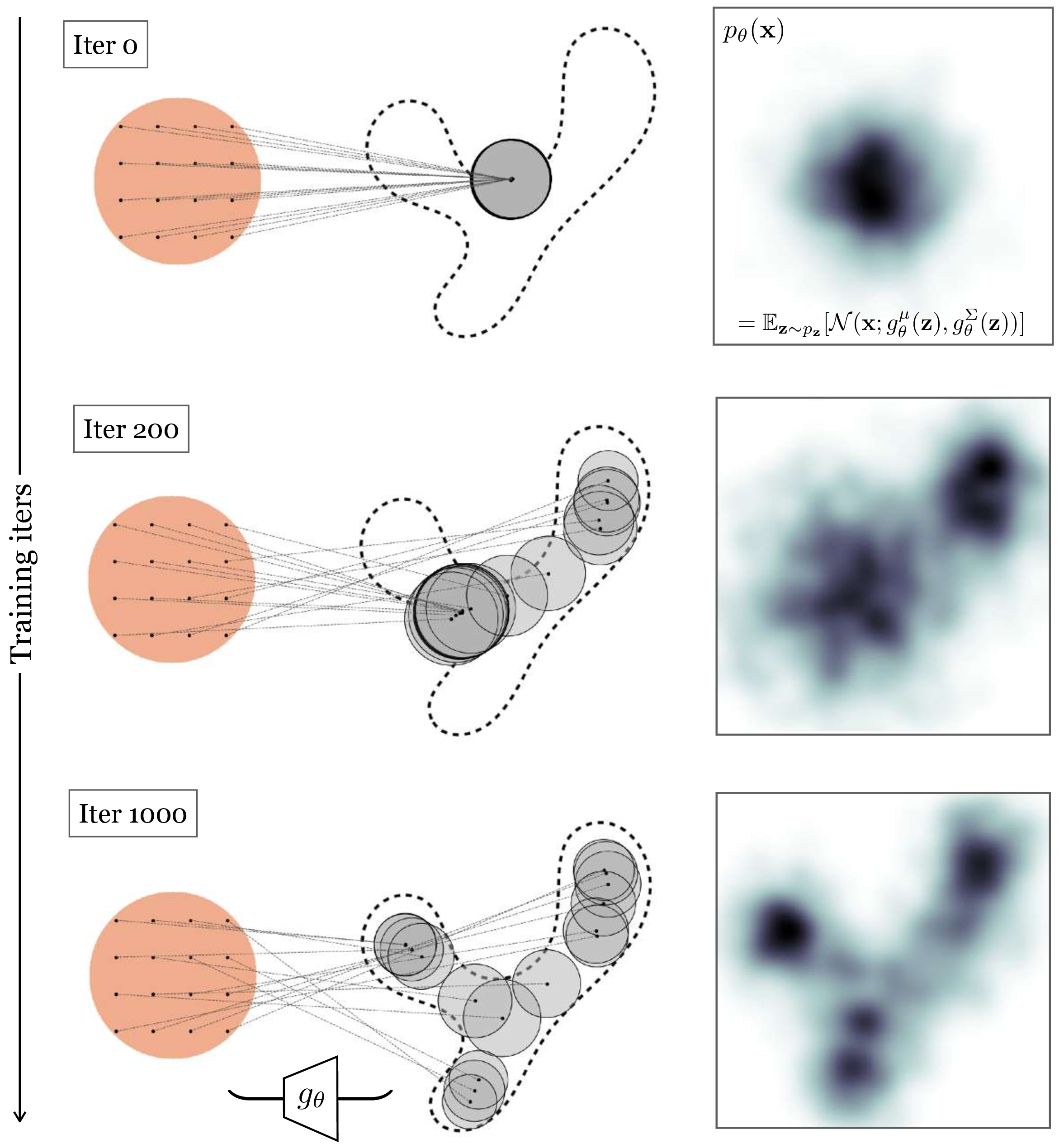
In Figure 33.6 we show what this process looks like at three checkpoints during training. Here we use an isotropic Gaussian model, that is, we parameterize the covariance as \(\Sigma = \sigma\mathbf{I}\), where \(\sigma = g^{\sigma}_{\theta}(\mathbf{z})\) is a scalar.
33.4.3.2 Trick 2: Efficient approximation via importance sampling
The previous trick works decently for modeling low-dimensional distributions. Unfortunately, this approach does not scale well to high-dimensions. The reason is that in order for our Monte Carlo estimate of the integral to be accurate, we may need many samples from \(p_{\mathbf{z}}\), and the higher the dimensionality of \(\mathbf{z}\), the more samples we will typically need.
Can we come up with a more efficient way of approximating the integral in Equation 33.3? Let’s start by writing out the sum from Equation 33.4 more explicitly:
\[\begin{aligned} p_{\theta}(\mathbf{x}) &\approx \frac{1}{M} (p_{\theta}(\mathbf{x} \bigm | \mathbf{z}^{(1)}) + p_{\theta}(\mathbf{x} \bigm | \mathbf{z}^{(2)}) + p_{\theta}(\mathbf{x} \bigm | \mathbf{z}^{(3)}) + \ldots) \end{aligned}\]
In general, some of the terms \(p_{\theta}(\mathbf{x} \bigm | \mathbf{z}^{(j)})\) will be larger than others. In fact, in our example in Figure 33.6, most of these terms are near zero. This is because, to maximize likelihood, the model spread out the Gaussians so that each places high density on a different part of the data distribution. A datapoint \(\mathbf{x}\) will only have substantial probability under the Gaussians whose means are near \(\mathbf{x}\).
Consider the example in Figure 33.7, where we are trying to esimate the probability of the point \(\mathbf{x}\) (blue circle).
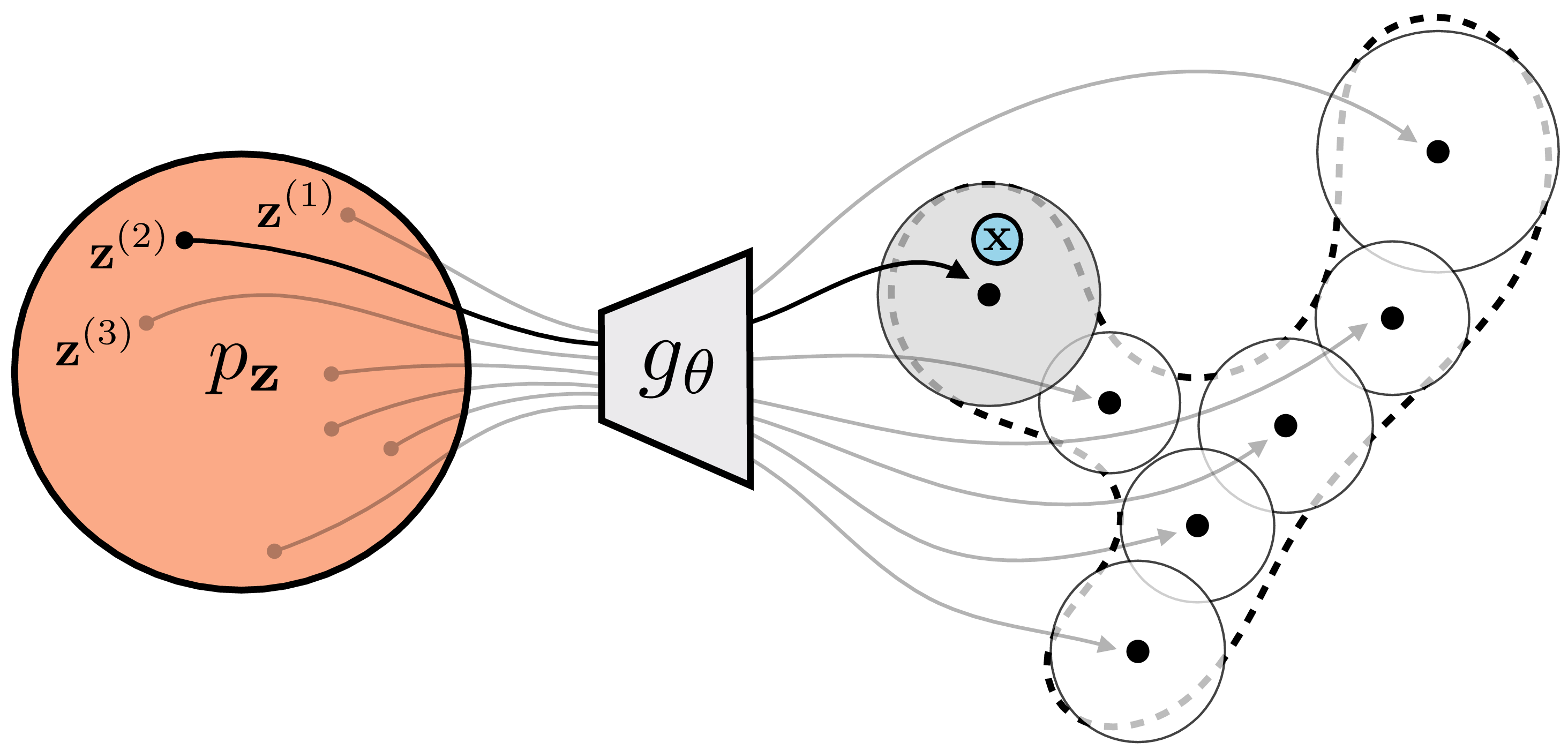
The mixture components are shaded according to the probability they assign to \(\mathbf{x}\). Almost all are so far from \(\mathbf{x}\) that we have: \[\begin{aligned} p_{\theta}(\mathbf{x}) &\approx \frac{1}{M} (0 + p_{\theta}(\mathbf{x} \bigm | \mathbf{z}^{(2)}) + 0 + \ldots) \end{aligned}\] If we had only sampled \(\mathbf{z}^{(2)}\), we would have had almost as good an estimate!
This brings us to the second trick of VAEs: when approximating the likelihood integral for \(p_{\theta}(\mathbf{x})\), try to only sample \(\mathbf{z}\) values that place high probability on \(\mathbf{x}\), that is, those \(\mathbf{z}\) values for which \(p_{\theta}(\mathbf{x} \bigm | \mathbf{z})\) is large. Then, a few samples will suffice to well approximate the entire expectation. This trick is called importance sampling. It is a general trick for approximating expectations. Rather than sampling \(\mathbf{z}^{(i)} \sim p_{\mathbf{z}}\), we sample from some other density \(\mathbf{z}^{(i)} \sim q_{\mathbf{z}}\), and multiply by a correction factor \(\frac{p_{\mathbf{z}}(\mathbf{z})}{q_{\mathbf{z}}(\mathbf{z})}\) to account for the fact that we are sampling from a biased distribution: \[\begin{aligned} p_{\theta}(\mathbf{x}) &= \mathbb{E}_{\mathbf{z}\sim p_{\mathbf{z}}}\Big[p_{\theta}(\mathbf{x} \bigm | \mathbf{z})\Big] = \int_{\mathbf{z}} p_{\mathbf{z}}(\mathbf{z}) p_{\theta}(\mathbf{x} \bigm | \mathbf{z}) d\mathbf{z} = \int_{\mathbf{z}} q_{\mathbf{z}}(\mathbf{z})\frac{p_{\mathbf{z}}(\mathbf{z})}{q_{\mathbf{z}}(\mathbf{z})} p_{\theta}(\mathbf{x} \bigm | \mathbf{z}) d\mathbf{z}\\ &= \mathbb{E}_{\mathbf{z}\sim q_{\mathbf{z}}}\Big[\frac{p_{\mathbf{z}}(\mathbf{z})}{q_{\mathbf{z}}(\mathbf{z})} p_{\theta}(\mathbf{x} \bigm | \mathbf{z})\Big] \end{aligned} \tag{33.6}\]
Using the intuition we developed previously, the distribution \(q\) we would really like to sample from is the one whose samples maximize \(p_{\theta}(\mathbf{x} \bigm | \mathbf{z})\). It turns out that the optimal distribution is \(q^* = p_{\theta}(Z \bigm | \mathbf{x})\).
See chapter 9, section 1 of [3] for a proof that \(q^*(\mathbf{z}) \propto \lvert p_{\theta}(\mathbf{x} \bigm | \mathbf{z}) \rvert p_{\mathbf{z}}(\mathbf{z})\), from which it then follows that \(q^*(\mathbf{z}) \propto p_{\theta}(\mathbf{x} \bigm | \mathbf{z})p_{\mathbf{z}}(\mathbf{z}) = p_{\theta}(\mathbf{x}, \mathbf{z}) \propto p_{\theta}(\mathbf{z} \bigm | \mathbf{x})\), yielding our result.
This distribution minimizes the expected error between a Monte Carlo estimate of the expectation and its true value (i.e., minimizes the variance of our Monte Carlo estimator). The intuition is that \(p_{\theta}(Z \bigm | \mathbf{x})\) is precisely a prediction of which \(\mathbf{z}\) values are most likely to have generated the observed \(\mathbf{x}\). The optimal importance sampling way to estimate the likelihood of a datapoint will therefore look like this: \[\begin{aligned} &p_{\theta}(\mathbf{x}) \approx \frac{1}{M} \sum_{j=1}^M\frac{p_{\mathbf{z}}(\mathbf{z}^{(j)})}{p_{\theta}(\mathbf{z}^{(j)} \bigm | \mathbf{x})} p_{\theta}(\mathbf{x} \bigm | \mathbf{z}^{(j)}) \quad\quad \triangleleft \quad\text{Optimal importance sampling}\\ &\quad\quad \mathbf{z}^{(j)} \sim p_{\theta}(Z \bigm | \mathbf{x}) \nonumber \end{aligned} \tag{33.7}\]
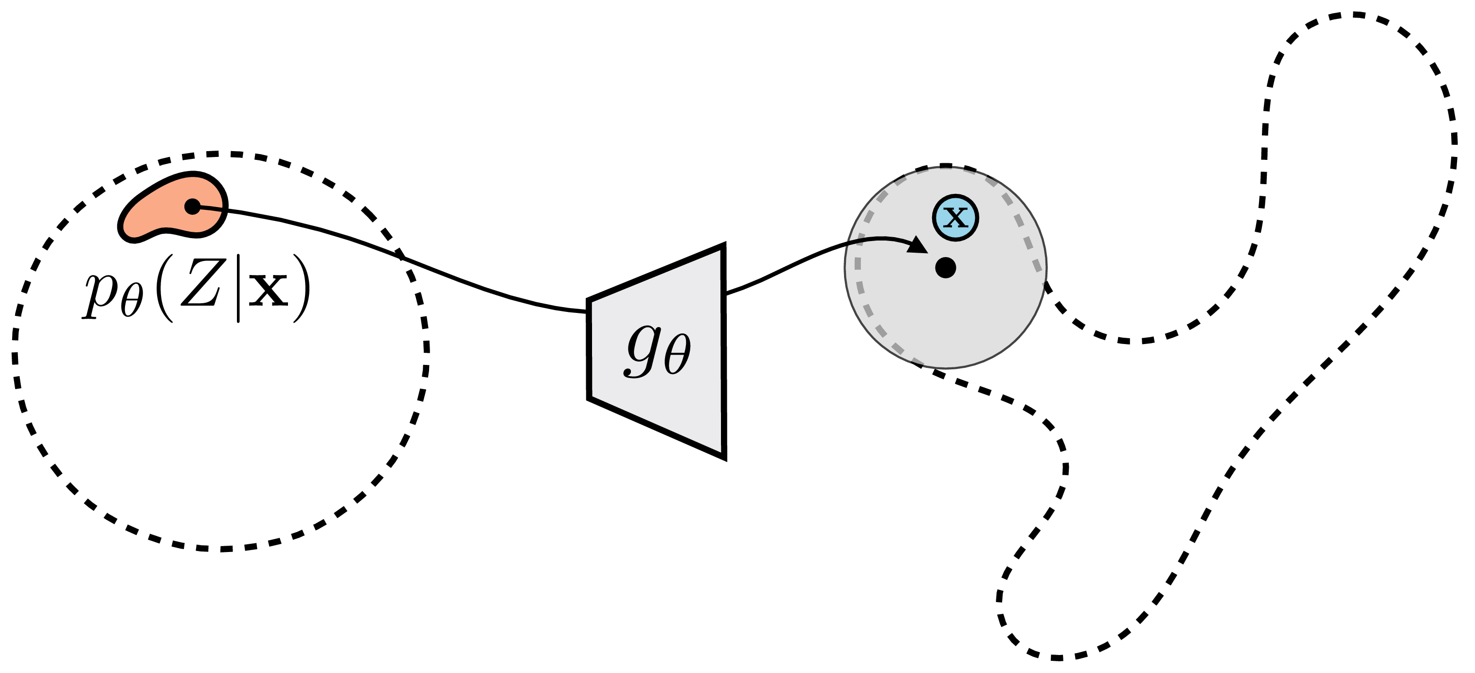
Visually, rather than sampling from all over \(p_{\mathbf{z}}\) and wasting samples on regions that place nearly zero likelihood on the data, we focus our sampling on just the region that places high likelihood on the data, and we can get then away with far fewer samples to well approximate the data likelihood, as indicated Figure 33.8.
33.4.3.3 Trick 3: Variational inference to approximate the sampling distribution
Now we know what distribution we should be sampling \(\mathbf{z}\) from: \(p_{\theta}(Z \bigm | \mathbf{x})\). The only remaining problem is that this distribution may be complicated and hard to sample from.
Remember, we have defined simple forms for only \(p_{\theta}(X \\| \mathbf{z})\) and \(p_{\mathbf{z}}\) (both are Gaussians), but this does not mean \(p_{\theta}(Z \\| \mathbf{x})\) has a simple form.
Sampling from arbitrary distributions is a standard topic in statistics, and many algorithms have been proposed, including the Markov chain Monte Carlo methods we encountered in previous chapters. VAEs use a strategy called variational inference.
The name variational comes from the “calculus of variations,” which studies functionals (functions of functions). Integrals of probability densities are functionals. Variational inference is commonly (but not always) used to approximate densities expressed as the integral of some other densities, hence functionals, hence the name variational.
The idea of variational inference is to approximate an intractable density \(p\) by finding the nearest density in a tractable family \(q_{\psi}\), parameterized by \(\psi\). In VAEs, we approximate our ideal importance density \(p_{\theta}(Z \bigm | \mathbf{x})\) with a \(q_{\psi}\) in a family we can efficiently sample from; the most common choice is to again use a Gaussian, conditioned on \(\mathbf{x}\): \(q_{\psi} = \mathcal{N}(f_{\psi}^{\mu}(\mathbf{x}), f_{\psi}^{\Sigma}(\mathbf{x}))\). The \(f_{\psi}\) is a function that maps from \(\mathbf{x}\) to parameters of a distribution over \(\mathbf{z}\); in other words, \(f_{\psi}\) is a probabilistic encoder! This function is shown next in Figure 33.9:
It will turn out that \(f\) indeed plays the role of the encoder in the VAE, while \(g\) plays the role of the decoder.
We want \(q_{\psi}\) to be the best approximation of \(p_{\theta}(Z \bigm | \mathbf{x})\), so our goal will be to choose the \(q_{\psi}\) that minimizes the Kullback-Leibler (KL) divergence between these two distributions. We could have chosen other divergences or notions of approximation, but we will see that using the KL divergence yields some nice properties. We will call the objective for \(q_{\psi}\) as \(J_{q}\), which we will define as the negative KL-divergence, so our goal is to maximize this quantity. Using the definition of KL-divergence, we can expand this objective as follows: \[\begin{aligned} J_q(\mathbf{x},\psi) &= -\mathrm{KL}\left(q_\psi(Z \mid \mathbf{x}) \| p_\theta(Z \mid \mathbf{x})\right)\\ &= -\mathbb{E}_{\mathbf{z} \sim q_{\psi}(Z \bigm | \mathbf{x})}[ \log q_{\psi}(\mathbf{z} \bigm | \mathbf{x}) - \log p_{\theta}(\mathbf{z} \bigm | \mathbf{x})]\\ &= -\mathbb{E}_{\mathbf{z} \sim q_{\psi}(Z \bigm | \mathbf{x})}[ \log q_{\psi}(\mathbf{z} \bigm | \mathbf{x}) - \log p_{\theta}(\mathbf{x} \bigm | \mathbf{z}) - \log p_{\mathbf{z}}(\mathbf{z}) + \log p_{\theta}(\mathbf{x})]\\ &= \mathbb{E}_{\mathbf{z} \sim q_{\psi}(Z \bigm | \mathbf{x})}[ -\log q_{\psi}(\mathbf{z} \bigm | \mathbf{x}) + \log p_{\theta}(\mathbf{x} \bigm | \mathbf{z}) + \log p_{\mathbf{z}}(\mathbf{z})] - \log p_{\theta}(\mathbf{x}) \end{aligned}\] The last line follows from the fact that \(\log p_{\theta}(\mathbf{x})\) is a constant with respect to the distribution we are taking expectation over.
The learning problem for \(q_{\psi}\) is to maximize \(J_q\), over all images in our dataset, \(\{\mathbf{x}^{(i)}\}_{i=1}^N\), with respect to parameters \(\psi\). Notice that the term \(\log p_{\theta}(\mathbf{x})\) is constant with respect to these parameters, so we can drop that term, yielding: \[\begin{aligned} \psi^* &= \mathop{\mathrm{arg\,max}}_{\psi} \frac{1}{N}\sum_{i=1}^N J_q(\mathbf{x}^{(i)}, \psi)\\ &= \mathop{\mathrm{arg\,max}}_{\psi} \frac{1}{N}\sum_{i=1}^N \underbrace{\mathbb{E}_{\mathbf{z} \sim q_{\psi}(Z \bigm | \mathbf{x}^{(i)})}[ -\log q_{\psi}(\mathbf{z} \bigm | \mathbf{x}^{(i)}) + \log p_{\theta}(\mathbf{x}^{(i)} \bigm | \mathbf{z}) + \log p_{\mathbf{z}}(\mathbf{z})]}_{J} \end{aligned} \tag{33.8}\] Here we have defined a new cost function, \(J\) (the term inside the sum in Equation 33.8), whose maximizer with respect to \(\psi\) is the same as the maximizer for \(J_q\).
Now, let us now recall our learning problem for \(p_{\theta}\), which is to maximize data log likelihood. Using importance sampling to estimate data likelihood (Equation 33.6, and using \(q_{\psi}\) as our sampling distribution, we have that the objective for \(p_{\theta}\) is to maximize the following objective \(J_p\) with respect to \(\theta\):
\[\begin{aligned} J_p(\mathbf{x},\theta) &= \log \mathbb{E}_{\mathbf{z}\sim q_{\psi}(Z \bigm | \mathbf{x})}\Big[\frac{p_{\mathbf{z}}(\mathbf{z})}{q_{\psi}(\mathbf{z} \bigm | \mathbf{x})} p_{\theta}(\mathbf{x} \bigm | \mathbf{z})\Big]\\ \theta^* &= \mathop{\mathrm{arg\,max}}_{\theta} \frac{1}{N}\sum_{i=1}^N J_p(\mathbf{x}^{(i)}, \theta) \end{aligned} \tag{33.9}\]
We now have a differentiable objective for both \(\psi\) and \(\theta\); the objective for \(\psi\) is expressed as an expectation and can be optimized by taking a Monte Carlo sample from that expectation. We could also try using Monte Carlo to approximate the objective for \(\theta\), but this would yield a biased estimator of \(\theta\), since Equation 33.9 has the log outside the expectation.
The expression \(\log \frac{1}{N} \sum_i x_i\) is not an unbiased estimator of \(\log \mathbb{E}[x]\), hence a Monte Carlo estimate is not the best choice for Equation 33.9.
That might be okay (as the number of samples \(N\) goes to infinity, the bias goes to zero), but we can do better. To get around this issue, VAEs adopt the following strategy: rather than maximizing \(J_p\) with respect to \(p_{\theta}\), they maximize a lower-bound to \(J_p\), which is expressed purely as an expectation and yields unbiased Monte Carlo estimates. The particular lower-bound used is in fact \(J\): the same objective we used for optimizing \(\psi\) in Equation 33.8!
The fact that \(J\) is a lower-bound on \(J_p\) follows from Jensen’s inequality: \[\begin{aligned} J_p &= \log p_{\theta}(\mathbf{x})\\ &= \log \mathbb{E}_{\mathbf{z}\sim q_{\psi}(Z \bigm | \mathbf{x})}\Big[\frac{p_{\mathbf{z}}(\mathbf{z})}{q_{\psi}(\mathbf{z} \bigm | \mathbf{x})} p_{\theta}(\mathbf{x} \bigm | \mathbf{z})\Big]\\ &\geq \mathbb{E}_{\mathbf{z}\sim q_{\psi}(Z \bigm | \mathbf{x})}\Big[\log \big(\frac{p_{\mathbf{z}}(\mathbf{z})}{q_{\psi}(\mathbf{z} \bigm | \mathbf{x})} p_{\theta}(\mathbf{x} \bigm | \mathbf{z})\big)\Big] \quad\quad \triangleleft \quad\text{Jensen's inequality}\\ &= \mathbb{E}_{\mathbf{z}\sim q_{\psi}(Z \bigm | \mathbf{x})}\Big[-\log q_{\psi}(\mathbf{z} \bigm | \mathbf{x}) + \log p_{\theta}(\mathbf{x} \bigm | \mathbf{z}) + \log p_{\mathbf{z}}(\mathbf{z}) \Big]\\ &= J \quad\quad\triangleleft\quad\text{VAE objective}\\ &\Rightarrow \quad J \leq J_p \end{aligned} \tag{33.10}\]
This way our learning problem for both \(\theta\) and \(\psi\) share the same objective (which also saves computation) and can be stated simply as:
\[\begin{aligned} \theta^*, \psi^* = \mathop{\mathrm{arg\,max}}_{\theta, \phi} \frac{1}{N}\sum_{i=1}^N J(\mathbf{x}^{(i)}, \theta, \phi) \end{aligned}\]
The VAE objective, \(J\), is often called the Evidence Lower Bound or ELBO, because it is a lower-bound on the data log-likelihood (i.e. \(J_p\), which equals \(\log p_{\theta}(\mathbf{x})\)).
Using the definition of KL-divergence, we can also rewrite \(J\) as follows: \[\begin{aligned} J &= \mathbb{E}_{\mathbf{z}\sim q_{\psi}(Z \bigm | \mathbf{x})}\Big[\log p_{\theta}(\mathbf{x} \bigm | \mathbf{z}) \Big] - \mathrm{KL}\left(q_\psi(Z \mid \mathbf{x}) \| p_{\mathbf{z}}\right) \quad\quad\triangleleft\quad\text{VAE objective} \end{aligned} \tag{33.11}\]
In this form, the VAE objective is presented as the sum of two terms. The first term measures the data log likelihood when the latent variables are sampled from \(q_{\psi}\) and the second term measures the gap between \(q_{\psi}\) and the distribution of latent variables, \(p_{\mathbf{z}}\), which we actually should have been sampling from to obtain the correct estimate of \(p_{\theta}(\mathbf{x})\).
33.4.4 Connection to Autoencoders
You may have noticed that in the previous sections we made use of both an encoder \(f_{\psi}\) (which parameterizes \(q_{\psi}(Z \bigm | \mathbf{x})\)) and a decoder \(g_{\theta}\) (which parameterizes \(p_{\theta}(X \bigm | \mathbf{z})\)); it looks like we are using the two pieces of an autoencoder but what’s the exact connection?
We will derive the connection for a simple VAE on one-dimensional (1D) data with 1D latent space, that is, \(x \in \mathbb{R}\), \(z \in \mathbb{R}\). First let us define shorthand notation for the means and variances of the Gaussians parameterized by the encoder and decoder: \[\begin{aligned} \mu_z &= f^{\mu}_{\psi}(x), & \sigma^2_z &= f^{\Sigma}_{\psi}(x)\\ \mu_x &= g^{\mu}_{\theta}(z), & \sigma^2_x &= g^{\Sigma}_{\theta}(z) \end{aligned}\] Then the distributions involved in the VAE are as follows: \[\begin{aligned} p_z &= \mathcal{N}(0,1)\\ q_{\psi}(Z \bigm | x) &= \mathcal{N}(\mu_z, \sigma^2_z)\\ p_{\theta}(X \bigm | z) &= \mathcal{N}(\mu_x, \sigma^2_x) \end{aligned}\]
As shown in Equation 33.11, the VAE learning problem seeks to maximize the following objective: \[\begin{aligned} \frac{1}{N}\sum_{i=1}^N \Big( \underbrace{\mathbb{E}_{z\sim q_{\psi}(Z \bigm | x^{(i)})}\Big[ \log p_{\theta}(x^{(i)} \bigm | z) \Big]}_{\text{likelihood term}} - \underbrace{\mathrm{KL}\left(q_\psi\left(Z \mid x^{(i)}\right) \| p_z\right)}_{\text{KL term}} \Big) \end{aligned}\]
On each step of optimization, we compute this objective over a batch of datapoints, and then apply backpropagation to update the parameters to increase the objective.
For each datapoint \(x\), the KL term can be computed in closed form since it is between two normal distributions (see the appendix of [1] for a derivation):
\[\begin{aligned} \mathrm{KL}\left(q_\psi(Z \mid x) \| p_z\right)&=\operatorname{KL}\left(\mathcal{N}\left(\mu_z, \sigma_z^2\right) \| \mathcal{N}(0,1)\right)\\ &= \frac{1}{2}(\mu_z^2 + \sigma_z^2 - \log(\sigma_z^2) - 1) \end{aligned}\]
The other term, the likelihood term, will be approximated by sampling. For each datapoint \(x\), we will take just a single sample from this expectation, as this is often sufficient in practice. To do so, first we encode \(x\) to parameterize \(q_{\psi}(Z \bigm | x)\). Then we sample a \(z\) from \(q_{\psi}(Z \bigm | x)\). Finally we decode this \(z\) to parameterize \(p_{\theta}(X \bigm | z)\), and we measure the probability this distribution places on our observed input \(x\), as shown below:
\[\begin{aligned} \mu_z, \sigma^2_z &= f_{\psi}(x) & \quad\quad \triangleleft \quad\text{Encode $x$}\\ z &\sim \mathcal{N}(\mu_z, \sigma^2_z) & \quad\quad \triangleleft \quad\text{Sample $z$} \end{aligned} \tag{33.12}\]
\[\begin{aligned} \mu_x, \sigma^2_x &= g_{\theta}(z) & \quad\quad \triangleleft \quad\text{Decode $z$}&\\ \log p_{\theta}(x | z) &= \log \mathcal{N}(x; \mu_x, \sigma^2_x) &\\ &= \log\frac{1}{\sigma_x\sqrt{2\pi}} - \frac{\overbrace{(x - \mu_x)^2}^{\text{reconstruction error}}}{2\sigma_x^2} & \quad\quad \triangleleft \quad\text{Measure likelihood} \end{aligned} \tag{33.13}\]
In other words, we encode, then decode, then measure the reconstruction error between our original input and the output of the decoder; this looks just like an autoencoder, as shown in Figure 33.10!
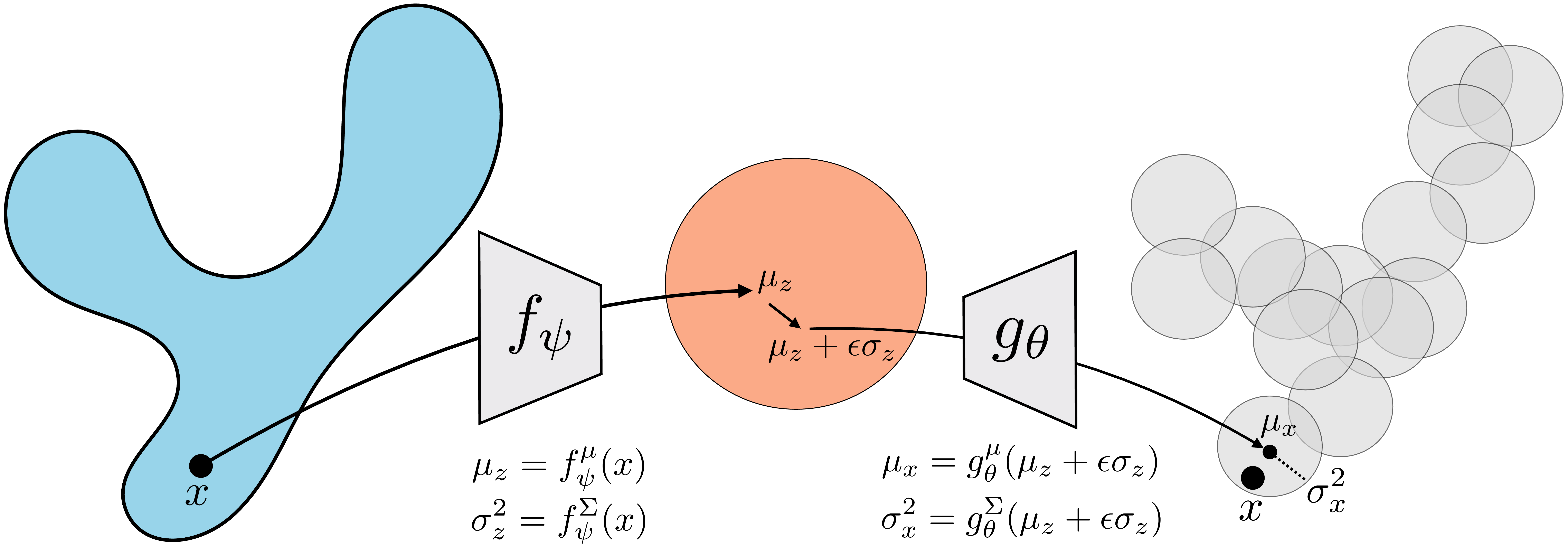
The only differences from an autoencoder are that 1) we sample a stochastic \(z\) from the output of the encoder, 2) the reconstruction error is scaled and offset by the predicted variance of the Gaussian likelihood model, and 3) we add to this term the KL loss defined previously.
Difference #1 is worth remarking on. To train the VAE, we need to backpropagate through the sampling step in Equation 33.12. How can we backpropagate through the sampling operation? The way to do this turns out to be quite simple: we reparameterize sampling from \(\mathcal{N}(\mu_z, \sigma^2_z)\) as follows:
\[\begin{aligned} \epsilon \sim \mathcal{N}(0,1)\\ z = \mu_z + \epsilon \sigma_z \end{aligned}\]
This step is known as the reparameterization trick, as it reparameterizes a stochastic function (sampling from a Gaussian parameterized by a neural net) to be a deterministic transformation of a fixed noise source (the unit Gaussian). To optimize the parameters for the encoder, we only need to backprogate through \(\mu_z\) and \(\sigma_z\), which are deterministic functions of \(x\), and therefore we have sidestepped the need to handle backpropagation through a stochastic function.
Putting all the terms together, the objective we are maximizing can now be written as:
\[\begin{aligned} \frac{1}{N}\sum_{i=1}^N \Big( \log\frac{1}{\sigma_{x^{(i)}}\sqrt{2\pi}} - \frac{\overbrace{(x^{(i)} - \mu_{x^{(i)}})^2}^{\text{reconstruction error}}}{2\sigma_{x^{(i)}}^2} - \underbrace{\frac{1}{2}(\mu_{z^{(i)}}^2 + \sigma_{z^{(i)}}^2 - \log(\sigma_{z^{(i)}}^2) - 1)}_{\text{KL term}} \Big) \end{aligned}\]
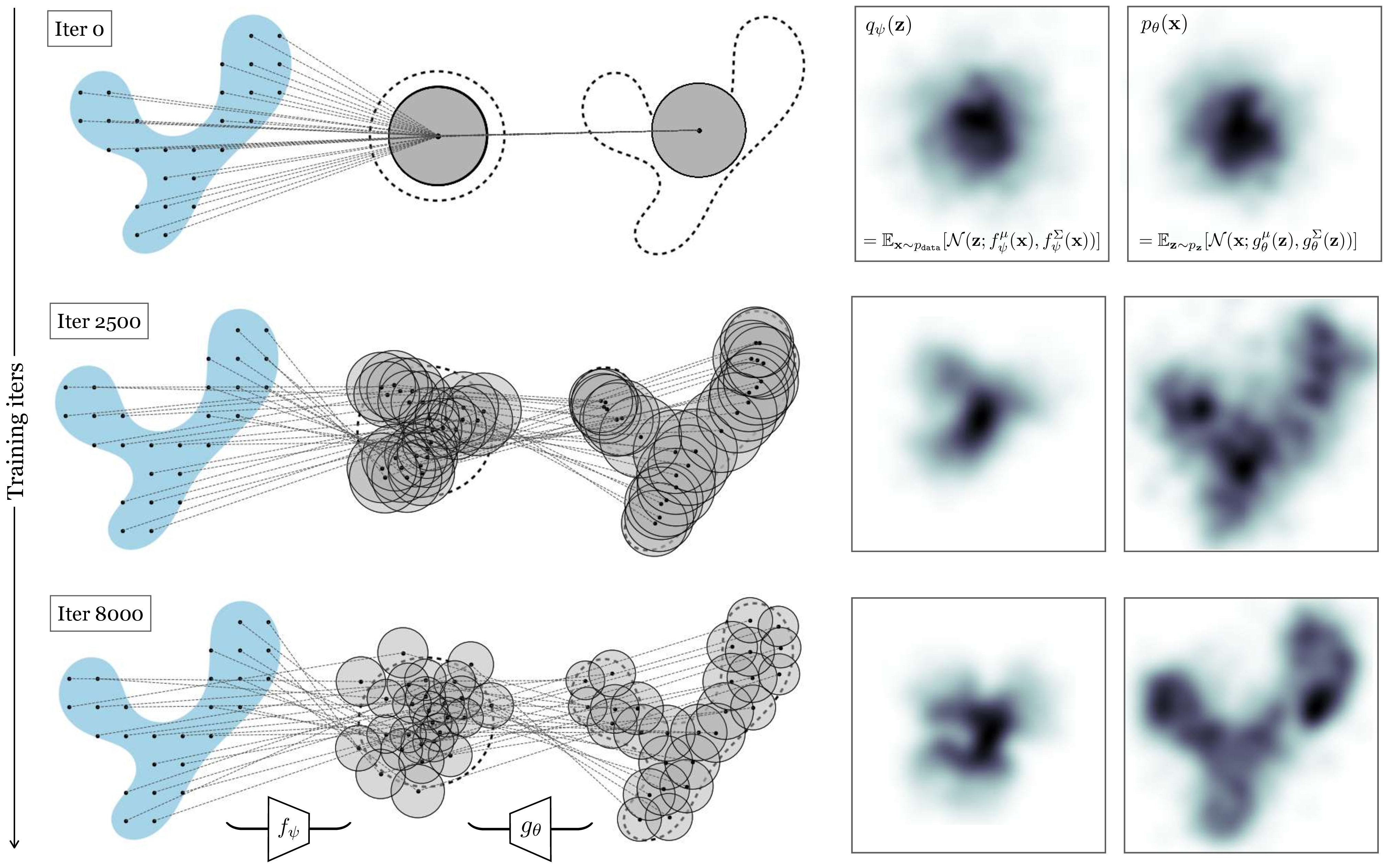
The KL term encourages the encodings \(z^{(i)}\) to be near a unit Gaussian distribution. To get an intuition for the effect of this term, consider the case where we fix \(\sigma_{z^{(i)}}\) to be 1; this is still a valid model for \(q_{\psi}(Z|x)\), just with lower capacity because it has fewer free parameters. In this simple case, the KL term reduces to \(\frac{1}{2}(\mu_{z^{(i)}}^2 - 1) \propto \mu_{z^{(i)}}^2\). The effect of this term is therefore to encourage the encodings \(\mu_{z^{(i)}}\) to be as close to zero as possible. In other words, the KL term squashes the distribution of latents (\(q_{\psi}(Z)\)) to be near the origin. Minimizing the reconstruction error, on the other hand, requires that the latents do not collapse to the origin; this term wants them to be as spread out as possible so as to preserve information about the inputs \(x^{(i)}\) that they encode. The tension between these two terms is what causes the VAE to work. While a standard autoencoder may produce an arbitrary latent distribution, with gaps and tendrils of density (as we saw in Figure 33.4), a VAE produces a tightly packed latent space which can be densely sampled from.
These effects can be seen in Figure 33.11, where we show three checkpoints of optimizing a VAE. As in the infinite mixture of Gaussians example shown previously, we again assume an isotropic Gaussian model for the decoder, and here also assume that model for the encoder.
33.5 Do VAEs Learn Good Representations?
One perspective on VAEs is that they are a way to train a generative model \(p_{\theta}\). From this perspective, the encoder is just scaffolding for learning a decoder. However, the encoder can also be useful as an end in itself, and we might instead think of the decoder as scaffolding for training an encoder. This was the perspective presented by autoencoders, after all, and the VAE encoder comes with the same useful properties: it maps data to a low-dimensional latent code that preserves information about the input. In fact, from a representation learning perspective, VAEs even go beyond autoencoders. Not only do VAEs learn a compressed embedding, the embeddings may also have other desirable properties depending on the prior \(p_{\mathbf{z}}\). For example, if \(p_{\mathbf{z}} = \mathcal{N}(0,1)\), as is common, then the loss encourages that the dimensions of the embedding are independent, a property called disentanglement.
Disentanglement means that we can vary one dimension of the embedding at time, and just one independent factor of variation in the generated images will change. For example, one dimension might control the direction of light in a scene and another dimension might control the intensity of light.
33.5.1 Example: Learning a VAE for Rivers
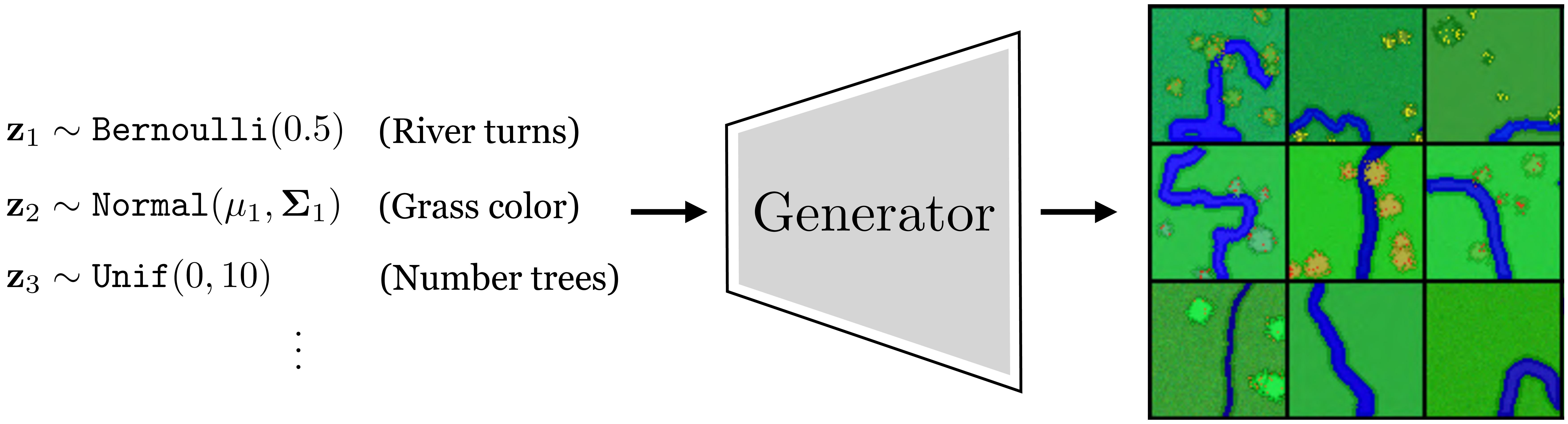
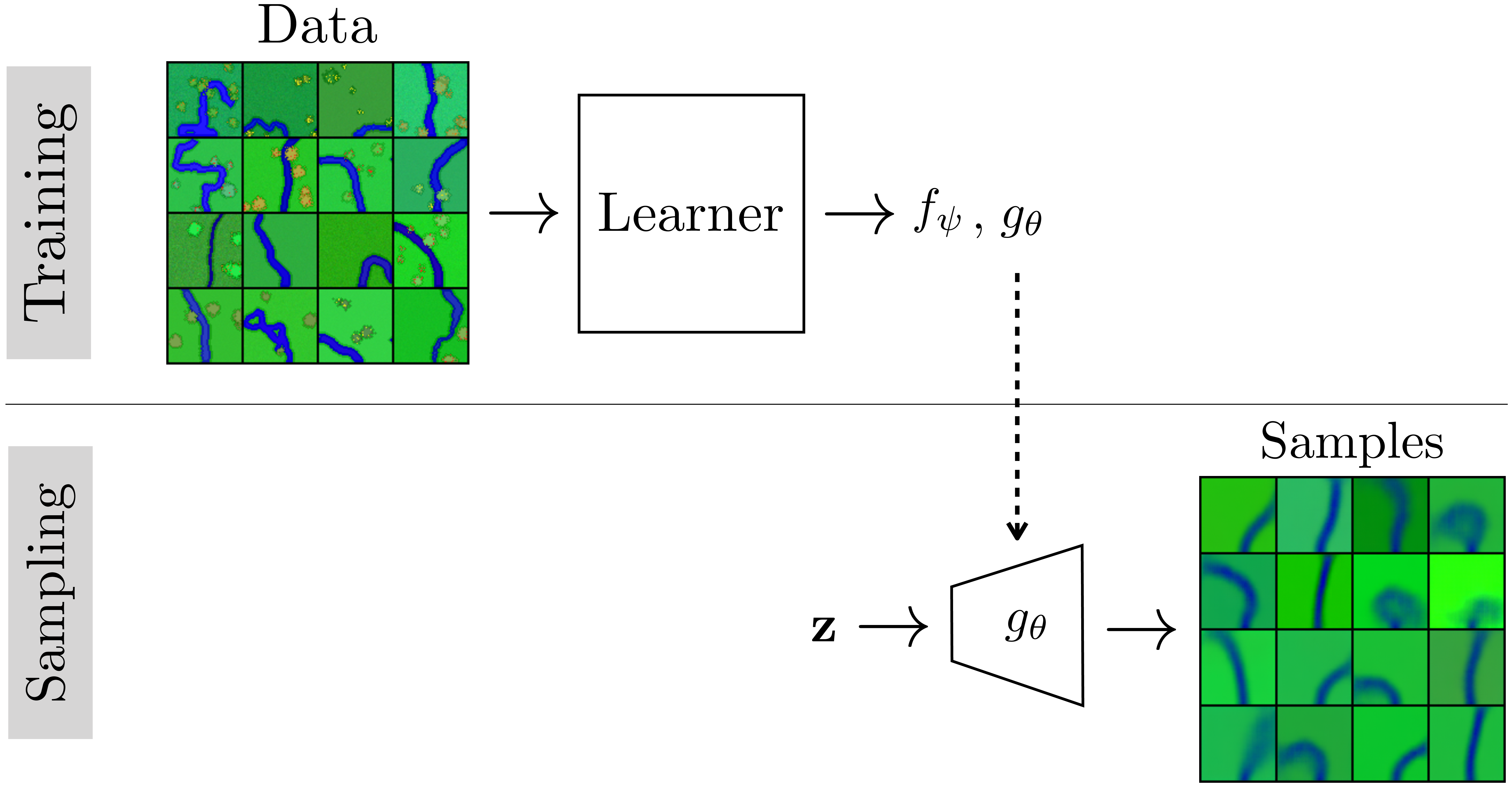
Suppose we have a dataset of aerial views of rivers. We wish to fit this data with a VAE so that (1) we can generate new rivers, and (2) we can identify the underlying latent variables that explain river appearance. In this example we will use data for which we know the true data generating process, which is simply a Python script that procedurally synthesizes cartoon images of rivers given input noise (this is a more elaborate version of the script we saw in Algorithm 32.1 of Chapter 32. The script takes in random values that control the attributes of the scene (the grass color, the heading of the river, the number of trees, etc.) and generates an image with these attributes, as shown in Figure 33.12.
Training a VAE on this data (Figure 33.13) learns to recreate the generative process with a neural net (rather than a Python script) and maps zero-mean unit-variance Gaussian noise to images (rather than taking as input the noise types the script uses).
Did the VAE uncover the true latent variables that generated the data, that is, did it recover latent dimensions corresponding to the attribute values that were the inputs to the Python script? We can examine this by generating a set of images that walk along two latent dimensions of the VAE’s \(z\)-space, shown in Figure 33.14.

One of the latent dimensions seems to control the grass color, and another controls the river curvature! These two latent dimensions are disentangled in the sense that varying the latent dimension that controls color has little effect on curvature and varying the latent dimension that controls curvature has little effect on color. Indeed, grass color was one of the attributes of the true data generating process (the Python script), and the VAE recovered it. However, interestingly there was no single input to the script that controls the overall river curvature, instead the curves are generating by a vector of Bernoulli variables that rotate the heading left and right as the river extends (using the same algorithm as in Algorithm 32.1.) The VAE has discovered a latent dimension that somehow summarizes a more global mode of behavior (i.e., bend left or bend right) than is explicit in the Python script. It is important to realize that VAEs, and most representation learning methods, do not necessarily recover the true causal mechanisms that generated the data but rather might find other mechanisms that can equivalently explain the data.
A formal name for this issue is the nonidentifiability of the true parameters that generated a dataset.
To summarize this section, we have seen that a VAE can be considered two things:
An efficient way to optimize an infinite mixture of Gaussians generative model.
A way to learn a low-dimensional, disentangled representation that can reconstruct the data.
33.6 Generative Adversarial Networks Are Representation Learners Too
In Chapter 32 we covered generative adversarial networks (GANs), which, like VAEs, train a mapping from latent variables to synthesized data, \(g: \mathbf{z} \rightarrow \mathbf{y}\). Do GANs also learn meaningful and disentangled latents?
To see, let us repeat the experiment of examining latent dimensions of a generative model, but this time with GANs. Here we will use a powerful GAN, called BigGAN [4], that has been trained on the ImageNet dataset [5]. Here are images generated by walking along two latent dimensions of this GAN (Figure 33.15):
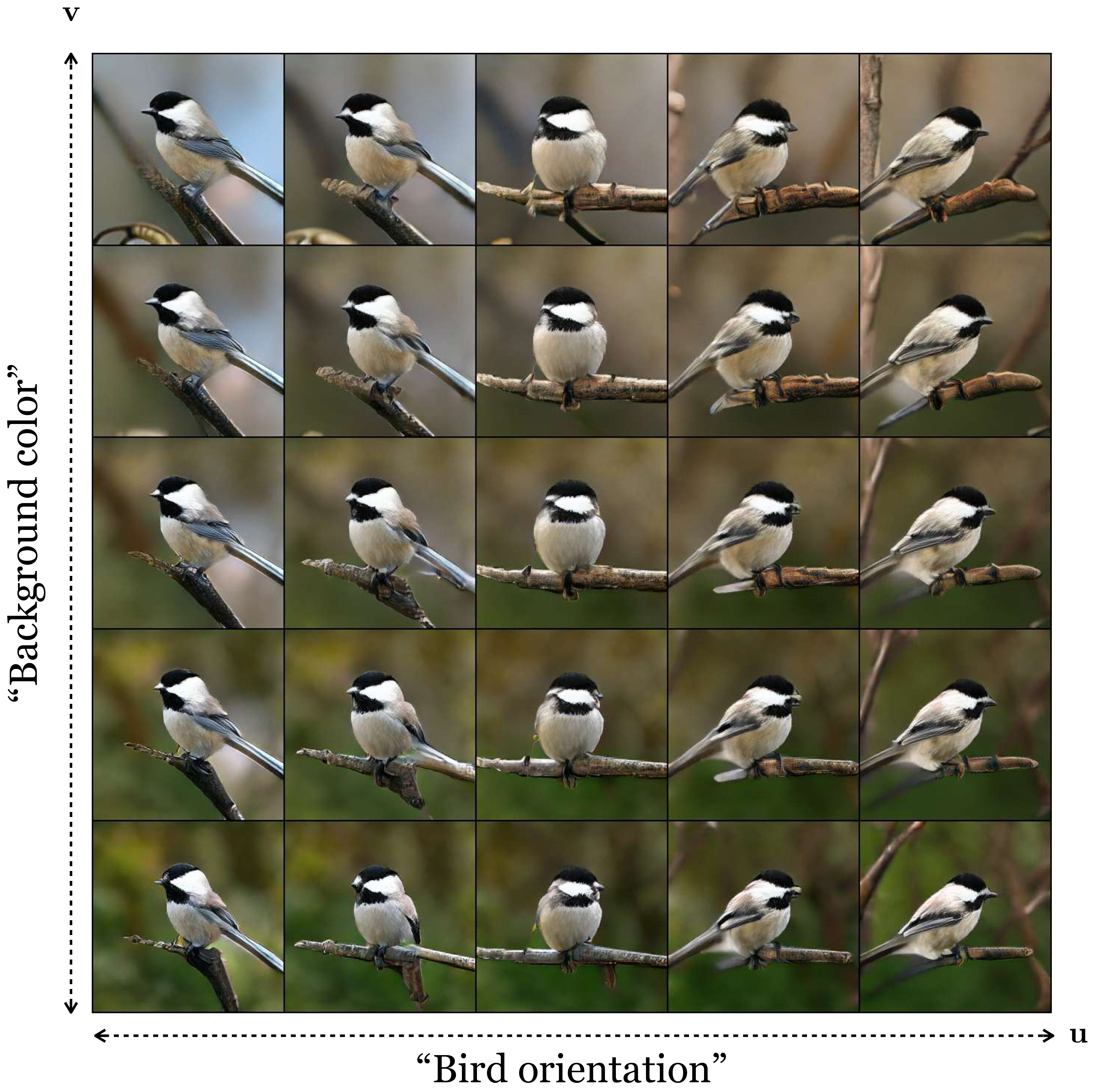
Just like with the VAE trained on cartoon rivers, the GAN has also discovered disentangled latent variables; in this case they seem to control background color and the bird’s orientation.
This makes sense: structurally, the GAN generator is very similar to the VAE decoder. In both cases, they map a low-dimensional random variable \(\mathbf{z}\) to data, and typically \(p_{\mathbf{z}} = \mathcal{N}(0,1)\). That means that the dimensions of \(\mathbf{z}\) are a priori independent (disentangled). In both models the goal is roughly the same: create synthetic data that has all the properties of real data. It should therefore come as no surprise that both models learn latent representations with similar properties. Indeed, these are just two examples of a large class of models that map low-dimensional latents from a simple (high entropy) distribution to high-dimensional data from a more structured (low entropy) distribution, and we might expect all models in this family to lead to similarly useful representations of the data.
33.7 Concluding Remarks
In this chapter we have seen that representation learning and generative modeling are intimately connected; they can be viewed as inverses of each other. This view also reveals an important property of the latent variables in generative models. These variables are like noise in that they are random variables with simple prior distributions, but they are not like our common sense understanding of noise as an unimportant nuisance. In fact, the latent variables can act as a powerful representation of the data. You may prefer to think of them as the underlying control knobs that generate the data. A user can spin these knobs randomly to get a random image, or they can tune the knobs navigate the natural image manifold in a systematic way, and arrive at the image they want.