14 Backpropagation
14.1 Introduction
A key idea of neural nets is to decompose computation into a series of layers. In this chapter we will think of layers as modular blocks that can be chained together into a computation graph. Figure 14.1 shows the computation graph for the two-layer multilayer perceptron (MLP) from chapter Chapter 12.

Each layer takes in some inputs and transforms them into some outputs. We call this the \(\texttt{forward}\) pass through the layer. If the layer has parameters, we will consider the parameters to be an input to a parameter-free transformation:
\[\begin{aligned} \mathbf{x}_{\texttt{out}}&= f(\mathbf{x}_{\texttt{in}},\theta) \end{aligned} \]
Graphically, we will depict the forward operation of a layer like shown below (Figure 14.2).
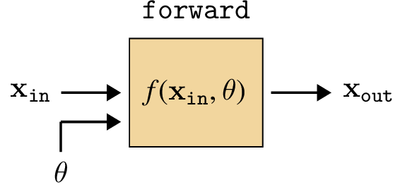
We will use the color to indicate free parameters, which are set via learning and are not the result of any other processing.
The learning problem is to find the parameters \(\theta\) that achieve a desired mapping. Usually, we will solve this problem via gradient descent. The question of this chapter is, how do we compute the gradients?
Backpropagation is an algorithm that efficiently calculates the gradient of the loss with respect to each and every parameter in a computation graph. It relies on a special new operation, called backward that, just like forward, can be defined for each layer, and acts in isolation from the rest of the graph. But first, before we get to defining backward, we will build up some intuition about the key trick backpropagation will exploit.
14.2 The Trick of Backpropagation: Reuse of Computation
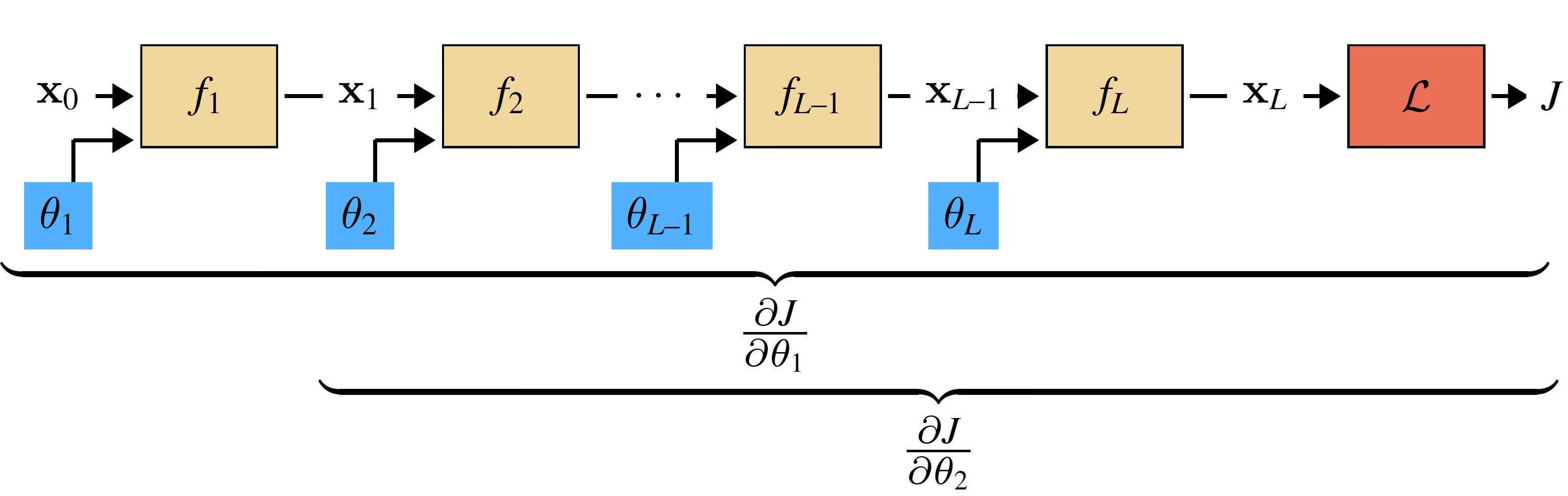
To start, we will consider a simple computation graph that is a chain of functions \(f_L \circ f_{L-1} \circ \cdots f_2 \circ f_1\), with each function \(f_l\) parameterized by \(\theta_l\).
Such a computation graph could represent an MLP, for example, which we will see in the next section.
We aim to optimize the parameters with respect to a loss function \(\mathcal{L}\). The loss can be treated as another node in our computation graph, which takes in \(\mathbf{x}_L\) (the output of \(f_L\)) and outputs a scalar \(J\), the loss. This computation graph appears as follows (Figure 14.3).
This computation graph is a narrow tree; the parameters live on branches of length 1. This can be easier to see when we plot it with data and parameters as nodes and edges as the functions: 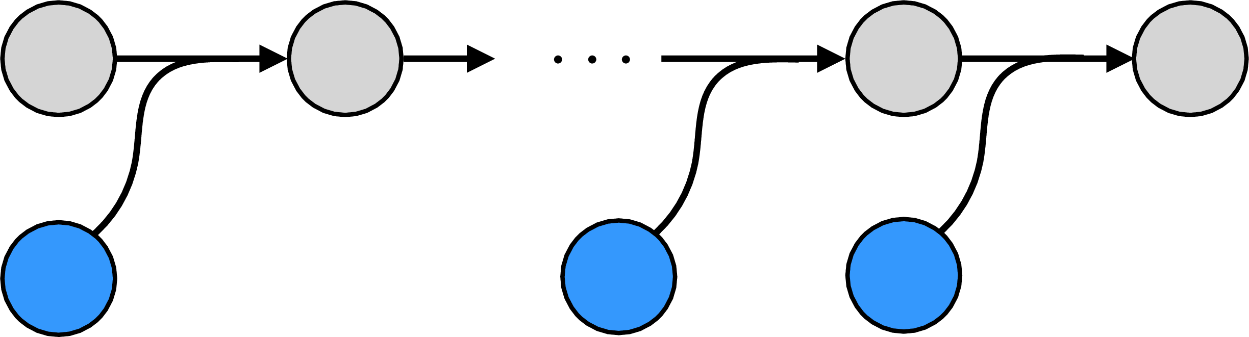 The parameters, along with the input training data, are the leaves of the computation graph.
Our goal is to update all the values highlighted in blue: \(\theta_1\), \(\theta_2\), and so forth. To do so we need to compute the gradients \(\frac{\partial J}{\partial \theta_1}\), \(\frac{\partial J}{\partial \theta_2}\), etc. Each of these gradients can be calculated via the chain rule. Here is the chain rule written out for the gradients for \(\theta_1\) and \(\theta_2\): \[ \begin{aligned} \frac{\partial J}{\partial \theta_1} &= % \colorbox{gray!20}{% $\displaystyle\mathstrut \frac{\partial J}{\partial \mathbf{x}_L} \frac{\partial \mathbf{x}_L}{\partial \mathbf{x}_{L-1}} \cdots \frac{\partial \mathbf{x}_3}{\partial \mathbf{x}_2} $% }% \, \frac{\partial \mathbf{x}_2}{\partial \mathbf{x}_1} \frac{\partial \mathbf{x}_1}{\partial \theta_1} \\ \frac{\partial J}{\partial \theta_2} &= % \colorbox{gray!20}{% $\displaystyle\mathstrut \frac{\partial J}{\partial \mathbf{x}_L} \frac{\partial \mathbf{x}_L}{\partial \mathbf{x}_{L-1}} \cdots \frac{\partial \mathbf{x}_3}{\partial \mathbf{x}_2} $% }% \, \frac{\partial \mathbf{x}_2}{\partial \theta_2} \end{aligned} \] Rather than evaluating both equations separately, we notice that most of the terms are shared. We only need to evaluate this product once, and then can use it to compute both \(\frac{\partial J}{\partial \theta_1}\) and \(\frac{\partial J}{\partial \theta_2}\). Now notice that this pattern of reuse can be applied in the same way for \(\theta_3\), \(\theta_4\), and so on. This is the whole trick of backpropagation: rather than computing each layer’s gradients independently, observe that they share many of the same terms, so we might as well calculate each shared term once and reuse them.
This strategy, in general, is called dynamic programming.
14.3 Backward for a Generic Layer
To come up with a general algorithm for reusing all the shared computation, we will first look at one generic layer in isolation, and see what we need in order to update its parameters (Figure 14.4).
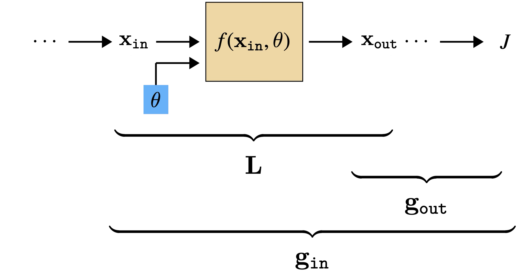
Here we have introduced two new shorthands, \(\mathbf{L}\) and \(\mathbf{g}\); these represent arrays of partial derivatives, defined below, and they are the key arrays we need to keep track of to do backprop. They are defined as:
\[\begin{aligned} \mathbf{g}_l&\triangleq \frac{\partial J}{\partial \mathbf{x}_l} &&\quad\quad \triangleleft \quad \text{grad of cost with respect to } \mathbf{x}_l \quad [1 \times |\mathbf{x}_l|]\\ \mathbf{L}&\triangleq \frac{\partial \mathbf{x}_{\texttt{out}}}{\partial [\mathbf{x}_{\texttt{in}}, \theta]} &&\quad\quad \triangleleft \quad \text{grad of layer}\\ &\quad\quad \mathbf{L}^{\mathbf{x}} \triangleq \frac{\partial \mathbf{x}_{\texttt{out}}}{\partial \mathbf{x}_{\texttt{in}}} &&\quad\quad \triangleleft \quad \text{\quad with respect to layer input data} \quad [|\mathbf{x}_{\texttt{out}}| \times |\mathbf{x}_{\texttt{in}}|]\\ &\quad\quad \mathbf{L}^{\theta} \triangleq \frac{\partial \mathbf{x}_{\texttt{out}}}{\partial \theta} &&\quad\quad \triangleleft \quad \text{\quad with respect to layer params} \quad [|\mathbf{x}_{\texttt{out}}| \times |\theta|] \end{aligned}\]
All these arrays represent the gradient at a single operating point, namely that of the current value of the data and parameters.
These arrays give a simple formula for computing the gradient we need, that is, \(\frac{\partial J}{\partial \theta}\), in order to update \(\theta\) to minimize the cost: \[\begin{aligned}
\frac{\partial J}{\partial \theta} &= \underbrace{\frac{\partial J}{\partial \mathbf{x}_{\texttt{out}}}}_{\mathbf{g}_{\texttt{out}}} \underbrace{\frac{\partial \mathbf{x}_{\texttt{out}}}{\partial \theta}}_{\mathbf{L}^{\theta}} = \mathbf{g}_{\texttt{out}}\mathbf{L}^{\theta}\\
\theta^{i+1} &\leftarrow \theta^{i} - \eta \Big(\frac{\partial J}{\partial \theta}\Big)^\mathsf{T}&&\quad\quad \triangleleft \quad \texttt{update}
\end{aligned} \tag{14.1}\]
The transpose is because, by convention, \(\theta\) is a column vector while \(\frac{\partial J}{\partial \theta}\) is a row vector; see the Notation section.
The remaining question is clear: how do we get \(\mathbf{g}_l\) and \(\mathbf{L}^{\theta}_l\) for each layer \(l\)?
Computing \(\mathbf{L}\) is an entirely local process: for each layer, we just need to know the functional form of its derivative, \(f^{\prime}\), which we then evaluate at the operating point \([\mathbf{x}_{\texttt{in}}, \theta]\) to obtain \(\mathbf{L}= f^{\prime}(\mathbf{x}_{\texttt{in}},\theta)\).
Computing \(\mathbf{g}\) is a bit trickier; it requires evaluating the chain rule, and depends on all the layers between \(\mathbf{x}_{\texttt{out}}\) and \(J\). However, this can be computed iteratively: once we know \(\mathbf{g}_l\), computing \(\mathbf{g}_{l-1}\) is just one more matrix multiply! This can be summarized with the following recurrence relation:
\[\begin{aligned} \mathbf{g}_{\texttt{in}} &= \mathbf{g}_{\texttt{out}}\mathbf{L}^{\mathbf{x}} &&\quad\quad \triangleleft \quad \text{backpropagation of errors} \end{aligned} \tag{14.2}\]
This recurrence is essence of backprop: it sends error signals (gradients) backward through the network, starting at the last layer and iteratively applying Equation 14.2 to compute \(\mathbf{g}\) for each previous layer.
Deep learning libraries like Pytorch have a field associated with each variable (data, activations, parameters). This field represents \(\frac{\partial J}{\partial v}\) for each variable \(v\).
We are finally ready to define the full backward function promised at the beginning of this chapter! It consists of the following operation, shown in Figure 14.5, which has three inputs (\(\mathbf{x}_{\texttt{in}}, \theta, \mathbf{g}_{\texttt{out}}\)) and two outputs (\(\mathbf{g}_{\texttt{in}}\) and \(\frac{\partial J}{\partial \theta}\)).
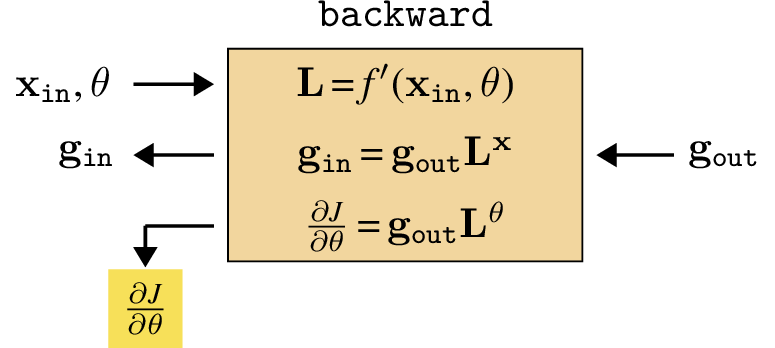
backward for a generic layer. We use the color to indicate parameter gradients.
We use the color for data/activation gradients being passed backward through the network.
14.4 The Full Algorithm: Forward, Then Backward
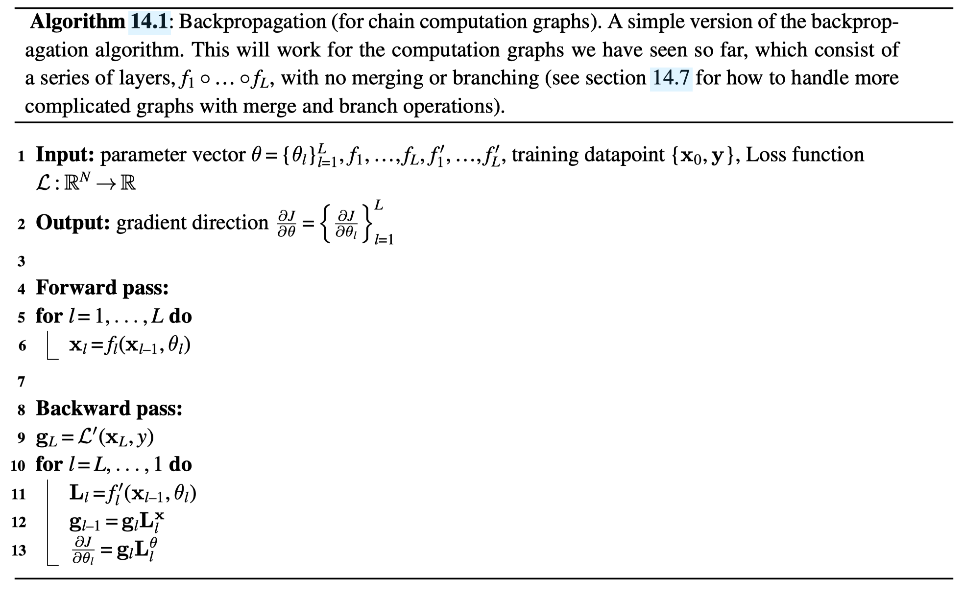
We are ready now to define the full backprop algorithm. In the last section we saw that we can easily compute the gradient update for \(\theta_l\) once we have computed \(\mathbf{L}_l\) and \(\mathbf{g}_l\).
The \(\mathbf{g}_l\) and \(\mathbf{L}_l\) are the \(\mathbf{g}\) and \(\mathbf{L}\) arrays for layer \(l\).
So, we just need to order our operations so that when we get to updating layer \(l\) we have these two arrays ready. The way to do it is to first compute a forward pass through the entire network, which means starting with input data \(\mathbf{x}_0\) and evaluating layer by layer to produce the sequence \(\mathbf{x}_0, \mathbf{x}_1, \ldots, \mathbf{x}_L\). Figure 14.6 shows what the forward pass looks like.

We use the color for data/activations being passed forward through the network.
Next, we compute a backward pass, iteratively evaluating the \(\mathbf{g}\)’s and obtaining the sequence \(\mathbf{g}_L, \mathbf{g}_{L-1}, \ldots\), as well as the parameter gradients for each layer (Figure 14.7).

The full algorithm is summarized in algorithm Algorithm 14.1.
14.5 Backpropagation Over Data Batches
So far, we have only examined computing the gradient of the loss for a single datapoint, \(\mathbf{x}\). As you may recall from Chapter 9 and Chapter 10, the total cost function we wish to minimize will typically be the average of the losses over all the datapoints in a training set, \(\{\mathbf{x}^{(i)}\}_{i=1}^N\).
However, once we know how to compute the gradient for a single datapoint, we can easily compute the gradient for the whole dataset, due to the following identity:
\[\begin{aligned} \frac{\partial \frac{1}{N}\sum_{i=1}^N J_i(\theta)}{\partial \theta} = \frac{1}{N} \sum_{i=1}^N \frac{\partial J_i(\theta)}{\partial \theta} \end{aligned} \tag{14.3}\]
The gradient of a sum of terms is the sum of the gradients of each term.
where \(J_i(\theta)\) is the loss for a single datapoint \(\mathbf{x}^{(i)}\). Therefore, to compute a gradient update for an algorithm like stochastic gradient descent Section 10.7, we apply backpropagation in batch mode, that is, we run it over each datapoint in our batch (which can be done in parallel) and then average the results.
In the remaining sections, we will still focus only on the case of backpropagation for the loss at a single datapoint. As you read on, keep in mind that doing the same for batches simply requires applying Equation 14.3.
The gradient of a sum of terms is the sum of the gradients of each term.
14.6 Example: Backpropagation for an MLP
In order to fully describe backprop for any given architecture, we need \(\mathbf{L}\) for each layer in the network. One way to do this is to define the derivative \(f^{\prime}\) for all atomic functions like addition, multiplication, and so on, and then expand every layer into a computation graph that involves just these atomic operations. Backprop through the expanded computation graph will then simply make use of all the atomic \(f^{\prime}\)s to compute the necessary \(\mathbf{L}\) matrices. However, often there are more efficient ways of writing backward for standard layers. In this section we will derive a compact backward for linear layers and relu layers — the two main layers in MLPs.
14.6.1 Backpropagation for a Linear Layer
The definition of a linear layer, in forward direction, is as follows: \[\begin{aligned} \mathbf{x}_{\texttt{out}}= \mathbf{W} \mathbf{x}_{\texttt{in}}+ \mathbf{b} \end{aligned}\] We have separated the parameters into \(\mathbf{W}\) and \(\mathbf{b}\) for clarity, but remember that we could always rewrite the following in terms of \(\theta = \texttt{vec}[\mathbf{W}, \mathbf{b}]\). Let \(\mathbf{x}_{\texttt{in}}\) be \(N\)-dimensional and \(\mathbf{x}_{\texttt{out}}\) be \(M\)-dimensional; then \(\mathbf{W}\) is an \([M \times N]\) dimensional matrix and \(\mathbf{b}\) is an \(M\)-dimensional vector.
Next we need the gradients of this function, with respect to its inputs and parameters, that is, \(\mathbf{L}\). Matrix algebra typically hides the details so we will instead first write out all the individual scalar gradients:
\[\begin{aligned} \mathbf{L}^{\mathbf{x}}[i,j] &= \frac{\partial x_{\texttt{out}}[i]}{\partial x_{\texttt{in}}[j]} = \frac{\partial \sum_l \mathbf{W}[i,l] x_{\texttt{in}}[l]}{\partial x_{\texttt{in}}[j]} = \mathbf{W}[i,j] \end{aligned} \tag{14.4}\]
\[\begin{aligned} \mathbf{L}^{\mathbf{W}}[i,jk] &= \frac{\partial x_{\texttt{out}}[i]}{\partial \mathbf{W}[j,k]} = \frac{\partial \sum_l \mathbf{W}[i,l] x_{\texttt{in}}[l]}{\partial \mathbf{W}[j,k]} = \begin{cases} x_{\texttt{in}}[k], &\text{if} \quad i == j\\ 0, & \text{otherwise} \end{cases} \label{lingrad2}\\ \mathbf{L}^{\mathbf{b}}[i,j] &= \frac{\partial x_{\texttt{out}}[i]}{\partial \mathbf{b}[j]} = \begin{cases} 1, &\text{if} \quad i == j\\ 0, & \text{otherwise} \end{cases} \end{aligned} \tag{14.5}\]
Equation 14.4 and Equation 14.5 imply:
\[\begin{aligned} \boxed{\mathbf{L}^{\mathbf{x}} = \mathbf{W}} &\quad\quad \triangleleft \quad [M \times N]\\ \boxed{\mathbf{L}^{\mathbf{b}} = \mathbf{I}} &\quad\quad \triangleleft \quad [M \times M] \end{aligned}\]
There is no such simple shorthand for \(\mathbf{L}^\mathbf{W}\), but that is no matter, as we can proceed at this point to implement backward for a linear layer by plugging our computed \(\mathbf{L}^\mathbf{x}\) into Equation 14.2, and \(\mathbf{L}^\mathbf{W}\) and \(\mathbf{L}^\mathbf{b}\) into Equation 14.1.
\[\begin{aligned} \mathbf{g}_{\texttt{in}} &= \mathbf{g}_{\texttt{out}}\mathbf{L}^{\mathbf{x}} = \mathbf{g}_{\texttt{out}}\mathbf{W}\\ \frac{\partial J}{\partial \mathbf{W}} &= \mathbf{g}_{\texttt{out}}\mathbf{L}^{\mathbf{W}}\\ \frac{\partial J}{\partial \mathbf{b}} &= \mathbf{g}_{\texttt{out}}\mathbf{L}^{\mathbf{b}} = \mathbf{g}_{\texttt{out}} \end{aligned} \tag{14.6}\]
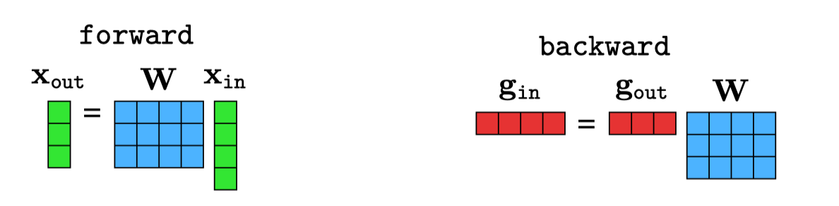
To get an intuition for Equation 14.6, it can help to draw the matrices being multiplied. Below, in Figure 14.8, on the left we have the forward operation of the layer (omitting biases) and on the right we have the backward operation in Equation 14.6.
Unlike the other equations, at first glance \(\frac{\partial J}{\partial \mathbf{W}}\) does not seem to have a simple form. A naive approach would be to first build out the large sparse matrix \(\mathbf{L}^{\mathbf{W}}\) (which is \([M \times MN]\), with zeros wherever \(i \neq k\) in \(\mathbf{L}^\mathbf{W}[i,jk]\)), then do the matrix multiply \(\mathbf{g}_{\texttt{out}}\mathbf{L}^{\mathbf{W}}\). We can avoid all those multiplications by zero by observing the following simplification:
\[\begin{aligned} \frac{\partial J}{\partial \mathbf{W}[i,j]} &= \frac{\partial J}{\partial \mathbf{x}_{\texttt{out}}} \frac{\partial \mathbf{x}_{\texttt{out}}}{\partial \mathbf{W}[i,j]} \quad\quad\quad\quad\quad\quad \triangleleft \quad[1 \times M][M \times 1] \rightarrow [1 \times 1]\\ &= \frac{\partial J}{\partial \mathbf{x}_{\texttt{out}}} \Big[\frac{\partial x_{\texttt{out}}[0]}{\partial \mathbf{W}[i,j]}, \ldots ,\frac{\partial x_{\texttt{out}}[M-1]}{\partial \mathbf{W}[i,j]} \Big]^\mathsf{T}\\ &= \frac{\partial J}{\partial \mathbf{x}_{\texttt{out}}} \Big[\ldots , 0, \ldots , \frac{\partial x_{\texttt{out}}[i]}{\partial \mathbf{W}[i,j]}, \ldots, 0, \ldots \Big]^\mathsf{T}\\ &= \frac{\partial J}{\partial \mathbf{x}_{\texttt{out}}} \Big[\ldots , 0, \ldots , x_{\texttt{in}}[j], \ldots, 0, \ldots \Big]^\mathsf{T}\\ &= \frac{\partial J}{\partial x_{\texttt{out}}[i]}x_{\texttt{in}}[j] \quad\quad\quad\quad\quad\quad \triangleleft \quad[1 \times 1][1 \times 1] \rightarrow [1 \times 1] \end{aligned}\]
In matrix equations, it’s very useful to check that the dimensions all match up. To the right of some equations in this chapter, we denote the dimensionality of the matrices in the product, where \(\mathbf{x}_{\texttt{in}}\) is M dimensions, \(\mathbf{x}_{\texttt{out}}\) is N dimensions, and the loss \(J\) is always a scalar.
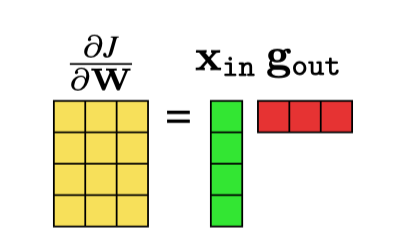
Now we can just arrange all these scalar derivatives into the matrix for \(\frac{\partial J}{\partial \mathbf{W}}\), and obtain the following: \[\begin{aligned} \frac{\partial J}{\partial \mathbf{W}} & = \begin{bmatrix} \frac{\partial J}{\partial \mathbf{W}[0,0]} & \ldots & \frac{\partial J}{\partial \mathbf{W}[N-1,0]} \\ \vdots & \ddots & \vdots \\ \frac{\partial J}{\partial \mathbf{W}[0,M-1]} & \ldots & \frac{\partial J}{\partial \mathbf{W}[N-1,M-1]} \\ \end{bmatrix}\\ & = \begin{bmatrix} \frac{\partial J}{\partial x_{\texttt{out}}[0]}x_{\texttt{in}}[0] & \ldots & \frac{\partial J}{\partial x_{\texttt{out}}[N-1]}x_{\texttt{in}}[0] \\ \vdots & \ddots & \vdots \\ \frac{\partial J}{\partial x_{\texttt{out}}[0]}x_{\texttt{in}}[M-1] & \ldots & \frac{\partial J}{\partial x_{\texttt{out}}[N-1]}x_{\texttt{in}}[M-1] \\ \end{bmatrix}\\ & = \mathbf{x}_{\texttt{in}}\frac{\partial J}{\partial \mathbf{x}_{\texttt{out}}}\\ &= \mathbf{x}_{\texttt{in}}\mathbf{g}_{\texttt{out}} \end{aligned}\]
Note, we are using the convention of zero-indexing into vectors and matrices.
So we see that in the end this gradient has the simple form of an outer product between two vectors, \(\mathbf{x}_{\texttt{in}}\) and \(\mathbf{g}_{\texttt{out}}\) (Figure 14.9).
We can summarize all these operations in the forward and backward diagram for linear layer in Figure 14.10.
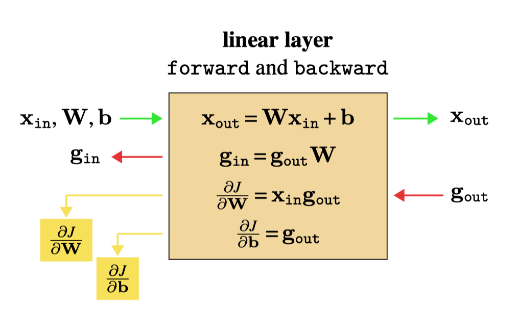
Notice that all these operations are simple expressions, mainly involving matrix multiplies. Forward and backward for a linear layer are also very easy to write in code, using any library that provides matrix multiplication (matmul) as a primitive. Figure 14.11 gives Python pseudocode for this layer.
class linear():
    def __init__(self, W, b, lr):
        self.W = W
        self.b = b
        self.lr = lr # learning rate

    def forward(self, x_in):
        self.x_in = x_in
        return matmul(W,x)+b

    def backward(self,J_out):
        J_in = matmul(J_out,W)
        dJdW = matmul(self.x_in,J_out)
        dJdb = J_out
        return J_in, dJdW, dJdb

    def update(self, dJdW, dJdb):
        self.W -= self.lr*dJdW.transpose()
self.b -= self.lr*dJdbforward and backward.
14.6.2 Backpropagation for a Pointwise Nonlinearity
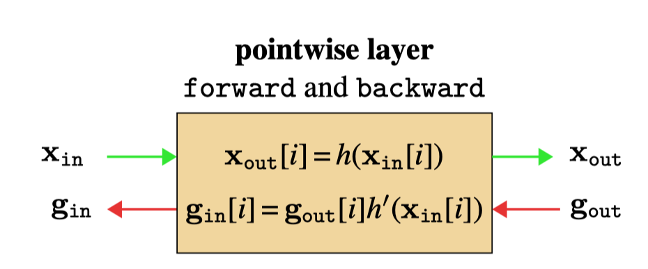
Pointwise nonlinearities have very simple backward functions. Let a (parameterless) scalar nonlinearity be \(h: \mathbb{R} \rightarrow \mathbb{R}\) with derivative function \(h^{\prime}: \mathbb{R} \rightarrow \mathbb{R}\). Define a pointwise layer using \(h\) as \(f(\mathbf{x}_{\texttt{in}}) = [h(x_{\texttt{in}}[0]), \ldots, h(x_{\texttt{in}}[N-1])]^\mathsf{T}\). Then we have \[\begin{aligned}
\mathbf{L}^{\mathbf{x}} &= f^{\prime}(\mathbf{x}_{\texttt{in}}) = \texttt{diag}([h^\prime(x_{\texttt{in}}[0]), \ldots, h^\prime(x_{\texttt{in}}[N-1])]^\mathsf{T}) \triangleq \mathbf{H}^\prime
\end{aligned}\]
The \(\texttt{diag}\) operator is the operator that places a vector on the diagonal of a matrix, whose other entries are all zero.
There are no parameters to update, so we just have to calculate \(\mathbf{g}_{\texttt{in}}\) in the backward operation, using Equation 14.2: \[\begin{aligned}
\mathbf{g}_{\texttt{in}} = \mathbf{g}_{\texttt{out}}\mathbf{H}^\prime
\end{aligned}\]
As an example, for a relu layer we have: \[\begin{aligned}
h^\prime(x) =
\begin{cases}
1 &\text{if} \quad x \geq 0\\
0 &\text{otherwise}
\end{cases}
\end{aligned}\] As a matrix multiply, the backward operation is shown in Figure 14.12.
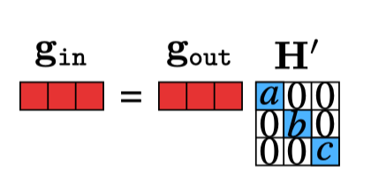
with \(a = h^\prime(x_{\texttt{in}}[0])\), \(b = h^\prime(x_{\texttt{in}}[1])\), and \(c = h^\prime(x_{\texttt{in}}[2])\). We can simplify this equation as follows:
\[\begin{aligned} \mathbf{g}_{\texttt{in}}[i] = \mathbf{g}_{\texttt{out}}[i]h^{\prime}(\mathbf{x}_{\texttt{in}}[i]) \quad \forall i \end{aligned} \tag{14.7}\]
The full set of operations for a pointwise layer is shown next in Figure 14.13.
14.6.3 Backpropagation for Loss Layers
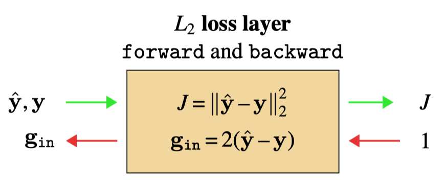
The last layer we need to define for a complete MLP is the loss layer. As a simple example, we will derive backprop for an \(L_2\) loss function: \(\left\lVert\hat{\mathbf{y}} - \mathbf{y}\right\rVert^2_2\), where \(\hat{\mathbf{y}}\) is the output of the network (prediction) and \(\mathbf{y}\) is the ground truth.
This layer has no parameters so we only need to derive Equation 14.2 for this layer: \[\begin{aligned} \mathbf{L}^{\mathbf{x}} &= \frac{\partial \left\lVert\hat{\mathbf{y}} - \mathbf{y}\right\rVert^2_2}{\partial \hat{\mathbf{y}}} = 2(\hat{\mathbf{y}} - \mathbf{y}) \quad\quad \triangleleft \quad [1 \times |\mathbf{y}|]\\ \mathbf{g}_{\texttt{in}} &= \mathbf{g}_{\texttt{out}}*2(\hat{\mathbf{y}} - \mathbf{y}) = 2(\hat{\mathbf{y}} - \mathbf{y}) \end{aligned}\] Here we have made use of the fact that \(\mathbf{g}_{\texttt{out}} = \frac{\partial J}{\partial \mathbf{x}_{\texttt{out}}} = \frac{\partial J}{\partial J} = 1\), since the output of the loss layer is the cost \(J\).
So, the backward signal sent by the \(L_2\) loss layer is a row vector of per-dimension errors between the prediction and the target.
This completes our derivation of \(\texttt{forward}\) and \(\texttt{backward}\) for a \(L_2\) loss layer, yielding Figure 14.14.
backward of an \(L_2\) loss layer.
14.6.4 Putting It All Together: Backpropagation through an MLP
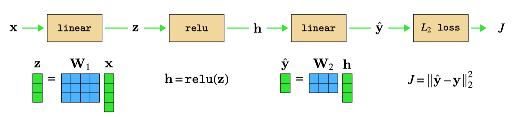
Let’s see what happens when we put all these operations together in an MLP. We will start with the MLP in Figure 14.1. For simplicity, we will omit biases. Let \(\mathbf{x}\) be four-dimensional and \(\mathbf{z}\) and \(\mathbf{h}\) be three-dimensional, and \(\hat{\mathbf{y}}\) be two-dimensional. The forward pass for this network is shown below in Figure 14.15.
For the backward pass, we will here make a slight change in convention, which will clarify an interesting connection between the forward and backward directions. Rather than representing gradients \(\mathbf{g}\) as row vectors, we will transpose them and treat them as column vectors. The backward operation for transposed vectors follows from the matrix identity that \((\mathbf{A}\mathbf{B})^\mathsf{T}= \mathbf{B}^\mathsf{T}\mathbf{A}^\mathsf{T}\): \[\begin{aligned}
\mathbf{g}^\mathsf{T}_{\texttt{in}} = (\mathbf{g}_{\texttt{out}}\mathbf{W})^\mathsf{T}= \mathbf{W}^\mathsf{T}\mathbf{g}^\mathsf{T}_{\texttt{out}}
\end{aligned}\]
Now we will draw the backward pass, using these transposed \(\mathbf{g}\)’s, in Figure 14.16.
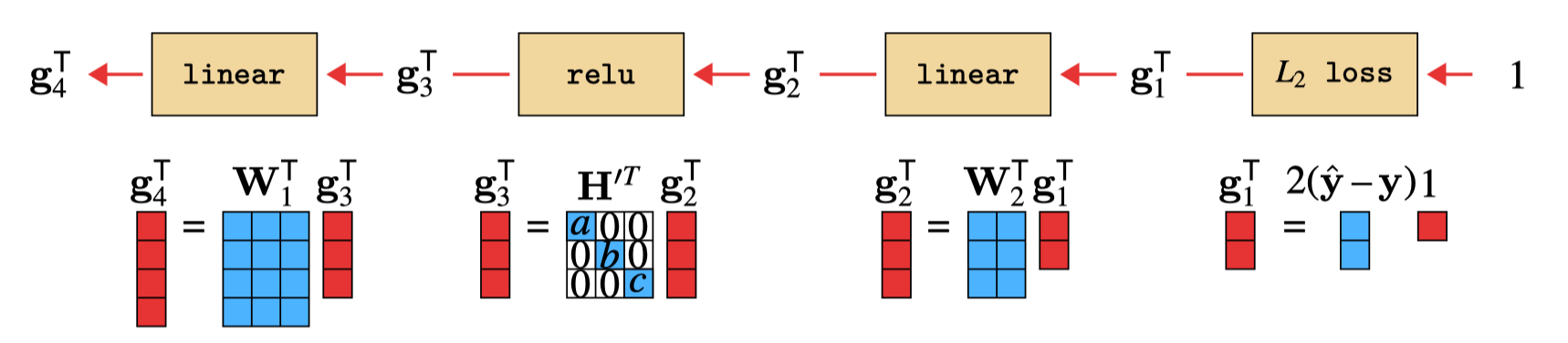
This reveals an interesting connection between forward and backward for linear layers: backward for a linear layer is the same operation as forward, just with the weights transposed! We have omitted the bias terms here, but recall from Equation 14.6 that the backward pass to the activations ignores biases anyway.
In contrast, the relu layer is not a relu on the backward pass. Instead, it becomes a sort of gating matrix, parameterized by functions of the activations from the forward pass (\(a\), \(b\), and \(c\)). This matrix is all zeros except for ones on the diagonal where the activation was nonnegative. This layer acts to mask out gradients for variables on the negative side of the \(\texttt{relu}\). Notice that this operation is a matrix multiply — in fact, all backward operations are matrix multiplies, no matter what the forward operation might be, as you can observe in algorithm Algorithm 14.1.
In the diagrams above, we have not yet included the computation of the parameter gradients. At each step of the backward pass, these are computed as an outerproduct between the activations input to that layer, \(\mathbf{x}_{\texttt{in}}\), and the gradients being sent back, \(\mathbf{g}_{\texttt{out}}\) (see Figure 14.9).
14.6.5 Forward-Backward Is Just a Bigger Neural Network
In the previous section we saw that the backward pass through an neural network can itself be implemented as another neural network, which is in fact a linear network with parameters determined by the weight matrices of the original network as well as by the activations in the original network. Therefore, the full backward pass is a neural network! Since the forward pass is also a neural network (the original network), the full backpropagation algorithm—a forward pass followed by a backward pass—can be viewed as just one big neural network. The parameter gradients can be computed from this network via one additional matrix multiply (matmul) for each layer of the backward network. The full network, for a three-layer MLP, is shown in Figure 14.17.
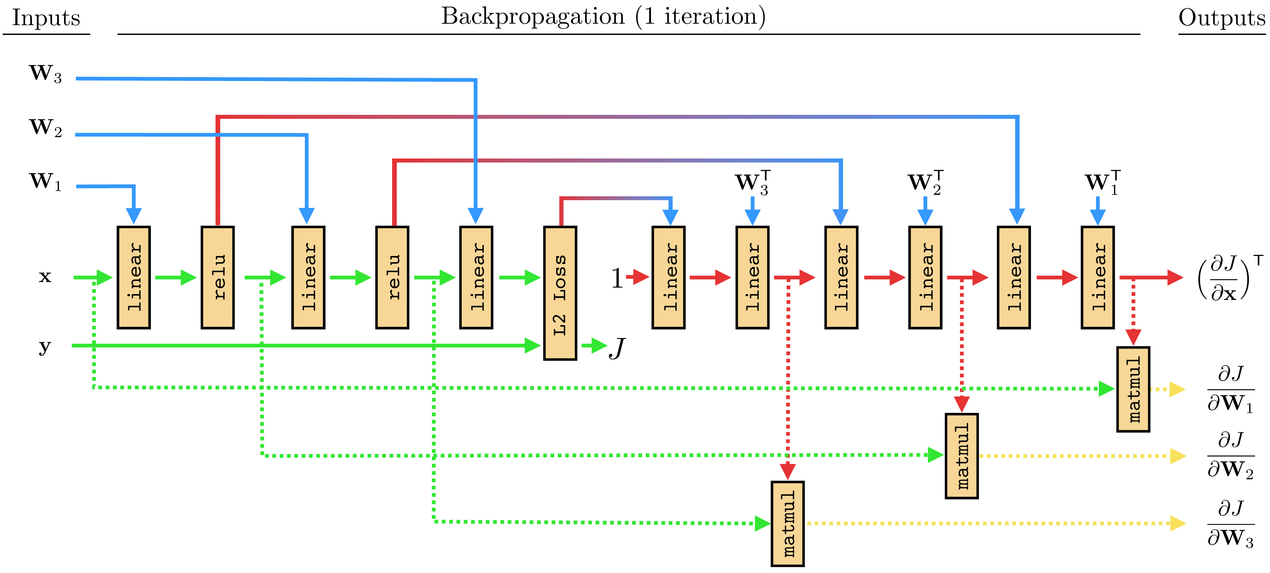
params forward params backward data forward data backward
There are a few interesting things about this forward-backward network. One is that activations from the relu layers get transformed to become parameters of a linear layer of the backward network (see Equation 14.7). There is a general term for this setup, where one neural net outputs values that parameterize another neural net; this is called a hypernetwork [1]. The forward network is a hypernetwork that parameterizes the backward network.
Another interesting property, which we already pointed out previously, is that the backward network only consists of linear layers. This is true no matter what the forward network consists of (even if it is not a conventional neural network but some arbitrary computation graph). The reason why this happens is because backprop implements the chain rule, and the chain rule is always a product of Jacobian matrices. Since a Jacobian is a matrix, clearly it is a linear function. But more intuitively, you can think of each Jacobian as being a locally linear approximation to the loss surface; hence each can be represented with a linear layer.
14.7 Backpropagation through DAGs: Branch and Merge
So far we have only seen chain-like graphs, –[]–[]–[]\(\rightarrow\). Can backprop handle other graphs? It turns out the answer is yes. Presently we will consider (DAGs). In Chapter 25, we will see that neural nets can also include cycles and still be trained with variants of backprop (e.g., backprop through time).
In a DAG, nodes can have multiple inputs and multiple outputs. In fact, we have already seen several examples of such nodes in the preceding sections. For example, a linear layer can be thought of as having two inputs, \(\mathbf{x}_{\texttt{in}}\) and \(\theta\), and one output \(\mathbf{x}_{\texttt{out}}\); or it can be thought of as having \(N = |\mathbf{x}_{\texttt{in}}| + |\theta|\) inputs and \(M = |\mathbf{x}_{\texttt{out}}|\) outputs, if we count up each dimension of the input and output vectors. So we have already seen DAG computation graphs.
However, to work with general DAGs, it helps to introduce two new special modules, which act to construct the topology of the graph. We will call these special operators merge and branch Figure 14.18.
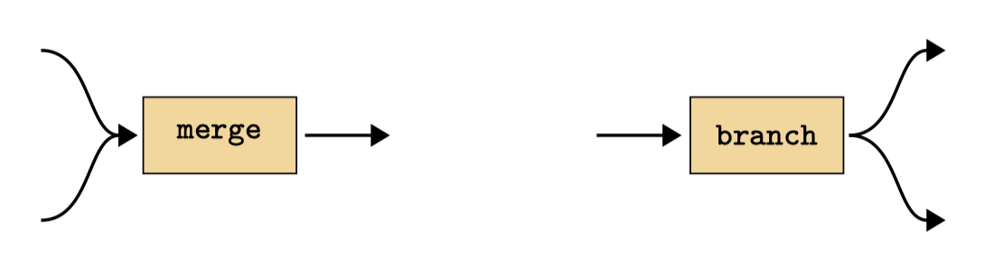
merge and branch layers.
We only consider binary branching and merging here, but branching and merging \(N\) ways can be done analogously or by repeating these operators.
We define them mathematically as variable concatenation and copying, respectively: \[\begin{aligned} \texttt{merge}(\mathbf{x}_{\texttt{in}}^a, \mathbf{x}_{\texttt{in}}^b) &\triangleq [\mathbf{x}_{\texttt{in}}^a, \mathbf{x}_{\texttt{in}}^b] \triangleq \mathbf{x}_{\texttt{out}}\\ \texttt{branch}(\mathbf{x}_{\texttt{in}}) &\triangleq [\mathbf{x}_{\texttt{in}}, \mathbf{x}_{\texttt{in}}] \triangleq [\mathbf{x}_{\texttt{out}}^a, \mathbf{x}_{\texttt{out}}^b] \end{aligned}\]
What if \(\mathbf{x}_{\texttt{in}}^a\) and \(\mathbf{x}_{\texttt{in}}^b\) are tensors, or other objects, with different shapes? Can we still concatenate them? The answer is yes. The shape of the data tensor has no impact on the math. We pick the shape just as a notational convenience; for example, it’s natural to think about images as two-dimensional arrays.
Here, \(\texttt{merge}\) takes two inputs and concatenates them. This results in a new multidimensional variable. The backward pass equation is trivial. To compute the gradient of the cost with respect to \(\mathbf{x}_{\texttt{in}}^{a}\), that is, \(\mathbf{g}_{\texttt{in}}^a\), we have \[\begin{aligned} \mathbf{g}_{\texttt{in}}^{a} &= \mathbf{g}_{\texttt{out}}\mathbf{L}^{\mathbf{x}^a} = \frac{\partial J}{\partial \mathbf{x}_{\texttt{out}}} \frac{\partial \mathbf{x}_{\texttt{out}}}{\partial \mathbf{x}_{\texttt{in}}^{a}}\\ %= \frac{\partial J}{\partial \mathbf{x}} \frac{\partial \texttt{merge}}{\partial \mathbf{x}^{a}}\\ &= \mathbf{g}_{\texttt{out}}\Big[\frac{\partial \mathbf{x}_{\texttt{in}}^{a}}{\partial \mathbf{x}_{\texttt{in}}^{a}}, \frac{\partial \mathbf{x}_{\texttt{in}}^{b}}{\partial \mathbf{x}_{\texttt{in}}^{a}}\Big]^\mathsf{T}\\ &= \mathbf{g}_{\texttt{out}}[1, 0]^\mathsf{T} \end{aligned}\] and likewise for \(\mathbf{g}_{\texttt{in}}^b\). That is, we just pick out the first half of the \(\mathbf{g}_{\texttt{out}}\) gradient vector for \(\mathbf{g}_{\texttt{in}}^a\) and the second half for \(\mathbf{g}_{\texttt{in}}^b\). There is really nothing new here. We already defined backpropagation for multidimensional variables above, and \(\texttt{merge}\) is just an explicit way of constructing multidimensional variables.
The branch operator is only slightly more complicated. In branching, we send copies of the same output to multiple downstream nodes. Therefore, we have multiple gradients coming back to the \(\texttt{branch}\) module, each from different downstream paths. So the inputs to this module on the backward pass are \(\frac{\partial J}{\partial \mathbf{x}_{\texttt{out}}^{a}}, \frac{\partial J}{\partial \mathbf{x}_{\texttt{out}}^{b}}\), which we can write as the gradient vector \(\mathbf{g}_{\texttt{out}}= \frac{\partial J}{\partial [\mathbf{x}_{\texttt{out}}^a, \mathbf{x}_{\texttt{out}}^b]} = [\frac{\partial J}{\partial \mathbf{x}_{\texttt{out}}^{a}}, \frac{\partial J}{\partial \mathbf{x}_{\texttt{out}}^{b}}] = [\mathbf{g}_{\texttt{out}}^a, \mathbf{g}_{\texttt{out}}^b]\). Let’s compute the backward pass output: \[\begin{aligned}
\mathbf{g}_{\texttt{in}}&= \mathbf{g}_{\texttt{out}}\mathbf{L}^{\mathbf{x}}\\
&= [\mathbf{g}_{\texttt{out}}^a, \mathbf{g}_{\texttt{out}}^b] \frac{\partial [\mathbf{x}_{\texttt{out}}^a, \mathbf{x}_{\texttt{out}}^b]}{\partial \mathbf{x}_{\texttt{in}}}\\
&= [\mathbf{g}_{\texttt{out}}^a, \mathbf{g}_{\texttt{out}}^b] \frac{\partial [\mathbf{x}_{\texttt{in}}, \mathbf{x}_{\texttt{in}}]}{\partial \mathbf{x}_{\texttt{in}}}\\
&= [\mathbf{g}_{\texttt{out}}^a, \mathbf{g}_{\texttt{out}}^b][1, 1]^\mathsf{T}\\
&= \mathbf{g}_{\texttt{out}}^a + \mathbf{g}_{\texttt{out}}^b
\end{aligned}\] So, branching just sums both the gradients passed backward to it.
Both \(\texttt{merge}\) and \(\texttt{branch}\) have no parameters, so there is no parameter gradient to define. Thus, we have fully specified the forward and backward behavior of these layers. The next diagrams summarize the behavior (Figure 14.19).
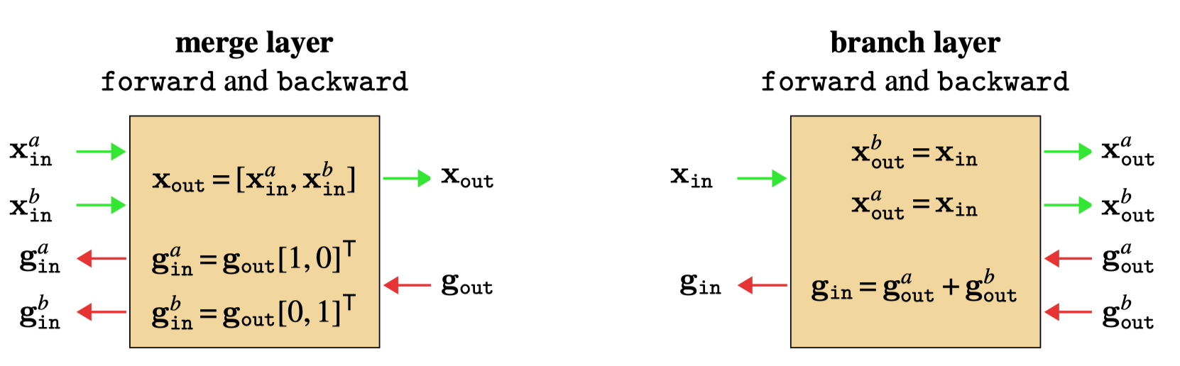
forward and backward.
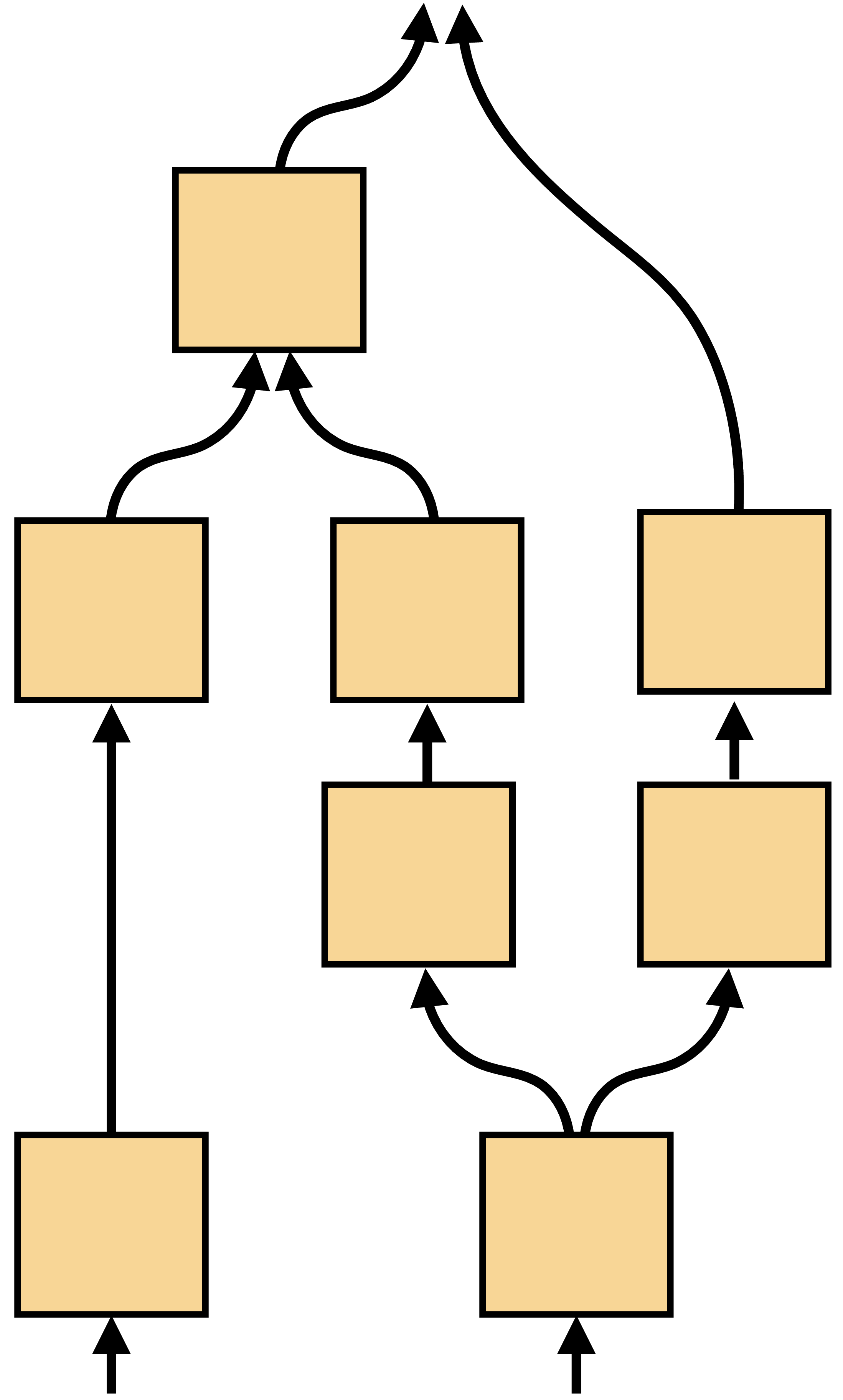
With merge and branch, we can construct any DAG computation graph by simply inserting these layers wherever we want a layer to have multiple inputs or multiple outputs. An example is given in Figure 14.20.
14.8 Parameter Sharing
Parameter sharing consists of a single parameter being sent as input to multiple different layers. We can consider this as a branching operation, as shown in Figure 14.21.
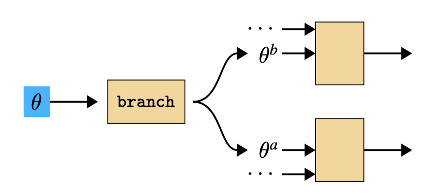
Then, from the previous section, it is clear that gradients summate for shared parameters. Let \(\{\theta^i\}^N_{i=1}\) be a set of variables that are all copies of one free parameter \(\theta\). Then, \[ \begin{aligned} \frac{\partial J}{\partial \theta} = \sum_i \frac{\partial J}{\partial \theta^i} \end{aligned} \]
14.9 Backpropagation to the Data
Backpropagation does not distinguish between parameters and data — it treats both as generic inputs to parameterless modules. Therefore, we can use backprop to optimize data inputs to the graph just like we can use backprop to optimize parameter inputs to the graph.
To see this, it helps to think about just the inputs and outputs to the full computation graph. In the forward direction, the inputs are the data and parameter settings and the output is the loss. In the backward direction, the input is the number 1 and the outputs are the are gradients of the loss with respect to the data and parameters. The full computation graph, for a learning problem using neural net \(F = f_L \circ \cdots \circ f_1\) and loss function \(\mathcal{L}\), is \(\mathcal{L}(F(\mathbf{x}_0), \mathbf{y}, \theta) \triangleq J(\mathbf{x}_0, \mathbf{y}, \theta)\). This function can itself be thought of as a single computation block, with inputs and outputs as specified previously (Figure 14.22).
In Pytorch you can only set input variables as optimization targets – these are called the leaves of the computation graph since, on the backward pass, they have no children. All the other variables are completely determined by the values of the input variables — they are not free variables.
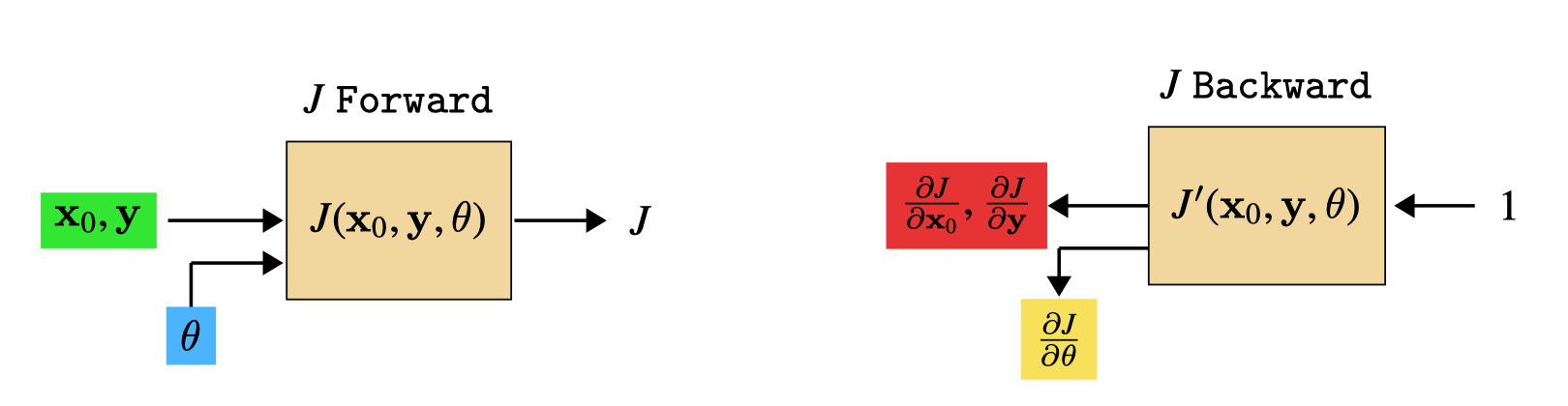
From this diagram, it should be clear that data inputs and parameter inputs play symmetric roles. Just as we can optimize parameters to minimize the loss, by descending the parameter gradient given by backward, we can also optimize input data to minimize the loss by descending the data gradient.
This can be useful for lots of different applications. One example is visualizing the input image that most activates a given neuron we are probing in a neural net. To do this, we define \(J\) to be the negative of the value of the neuron we are probing1, that is, \(J(\mathbf{x}_0,\theta) = -x_{l}[i]\) if we are interested in the \(i\)-th neuron on layer \(l\) (notice \(\mathbf{y}\) is not used for this problem). We show an example of this in Figure 14.23 below, where we used backprop to find the input image that most activates a node in the computation graph that scores whether or not an image is “a photo of a cat.” Do you see cat-like stuff in the optimized image? What does this tell you about how the network is working?
1 It is negative so that minimizing the loss maximizes the activation.
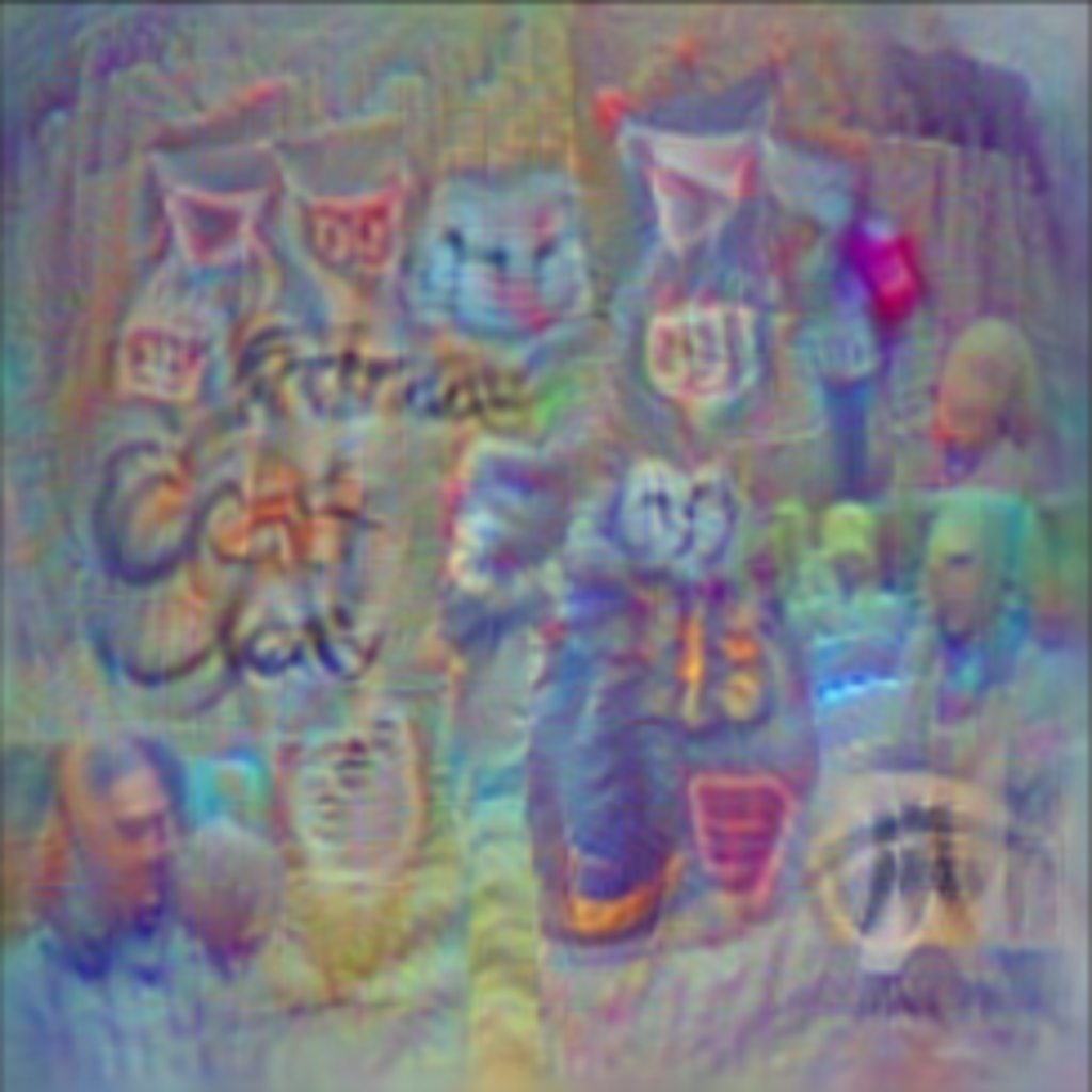
Visualizations like this are a useful way to figure out what visual features a given neuron is sensitive to. Researchers often combine this visualization method with a natural image prior in order to find an image that not only strongly activates the neuron in question but also looks like a natural photograph (e.g., [3]).
14.10 Concluding Remarks
Backprop is often presented as a method just for training neural networks, but it is actually a much more general tool than that. Backprop is an efficient way to find partial derivatives in computation graphs. It is general to a large family of computation graphs and can be used not just for learning parameters but also for optimizing data.