6 Lenses
6.1 Introduction
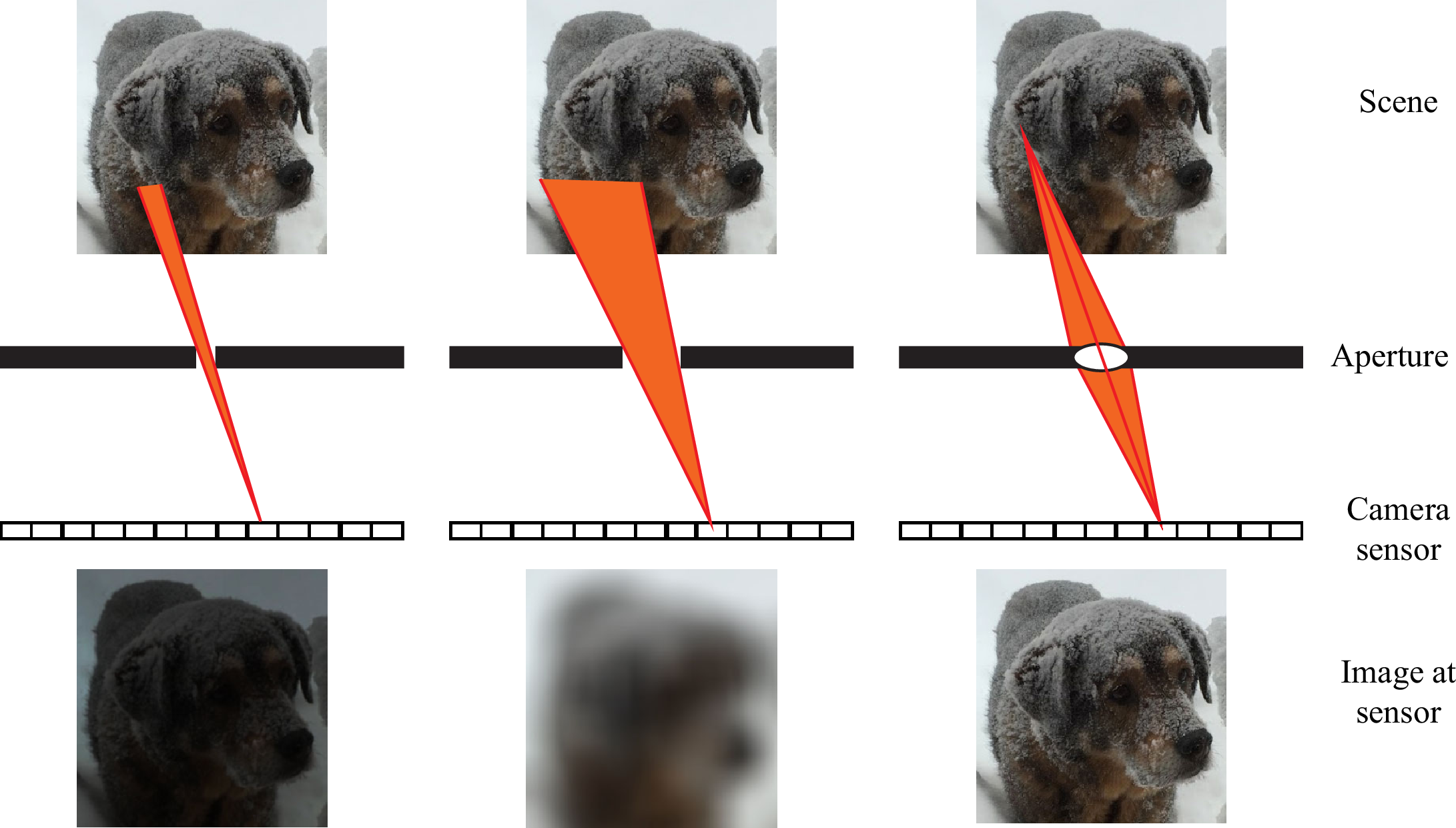
While pinhole cameras can form good images, they suffer from a serious drawback: the images are very dim because not much light passes through the small pinhole to the sensing plane of the pinhole camera. As shown in Figure 6.1 and Figure 6.2, one can try to let in more light by making the pinhole aperture bigger. But that allows light from many different positions to land on a given position at the sensor plane, resulting in a bright but blurry image. Putting a lens in the larger aperture can give the best of both worlds, capturing more light while redirecting the light rays entering the camera so that each sensor plane position maps to just one surface point, creating a focused image on the sensor plane. Here we analyze how light passes through lenses under the approximation of geometric optics, where we ignore effects like diffraction, due to the wave nature of light.
6.2 Lensmaker’s Formula
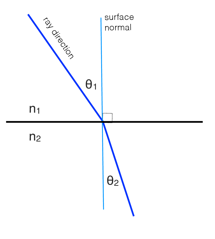
In general, light changes both its wavelength and its speed as it passes from one material to another. Those changes at the material interface will cause the light to bend, an effect called refraction. The amount of light bending depends on the change of speed of light within each material, and the orientation of the light ray with respect to the interface surface, according to Snell’s Law [1], given in the equation below. Both the wavelength and the speed of light in a medium are inversely proportional to the index of refraction of that medium, denoted as \(n\). The \(n\) for a vacuum is 1. At a material boundary, for the geometry illustrated in Figure 6.3, we have \[n_1 \sin(\theta_1) = n_2 \sin(\theta_2)\] where \(\theta_1\) and \(\theta_2\) are the angles with respect to the surface normal of the incident and outgoing light rays, and \(n_1\) and \(n_2\) are the indices of refraction of the materials in region 1 and region 2. Snell’s law can be derived by matching the wavelength of light projected along the material interface boundary across each side of the boundary.
Snell’s Law relates the bending angles of refraction, \(\theta_1\) and \(\theta_2\), to the indices of refraction, \(n_1\) and \(n_2\), at a material interface.
A lens is a specially shaped piece of transparent material, positioned to focus light from a surface point onto a sensor. In an ideal world, a lens focusing light from a surface onto a sensor plane has the property that every light ray from the surface point that passes through the lens is refracted onto a common position at the sensor, no matter what part of the lens the ray from the surface hits. This dramatically increases the light-gathering ability of the camera system, overcoming the poor light-gathering properties of a pinhole camera system.
To achieve that property, we must find a surface shape that allows for this focusing. Modern lens surfaces are designed by numerical optimization methods, trading off engineering constraints to achieve the best design, often involving several optical elements and different materials. But to gain insight into the properties of lenses, we can analytically design a lens surface shape provided we simplify the optical system.
For small angles \(\theta\) denoted in radians, \(\sin(\theta) \approx \theta\). If we also assume the index of refraction of air is 1 (it is 1.0003) and denote the index of refraction of lens glass as \(n\), then Snell’s law, as shown in Figure 6.3, becomes \[\theta_1 = n \theta_2,\] for small bending angles \(\theta_1\) and \(\theta_2\).
Consider a lens, and two points along its optical axis at a distance \(a\) and \(b\) from the lens, as shown in Figure 6.4 (a). We seek to find a surface shape for a lens which creates the light paths shown in Figure 6.4 (a): light leaving from any direction at point \(a\) will be focused to arrive at point \(b.\) Figure 6.4 (b) shows a view of Figure 6.4 (a), with angles and distances distorted for clarity of labeling.
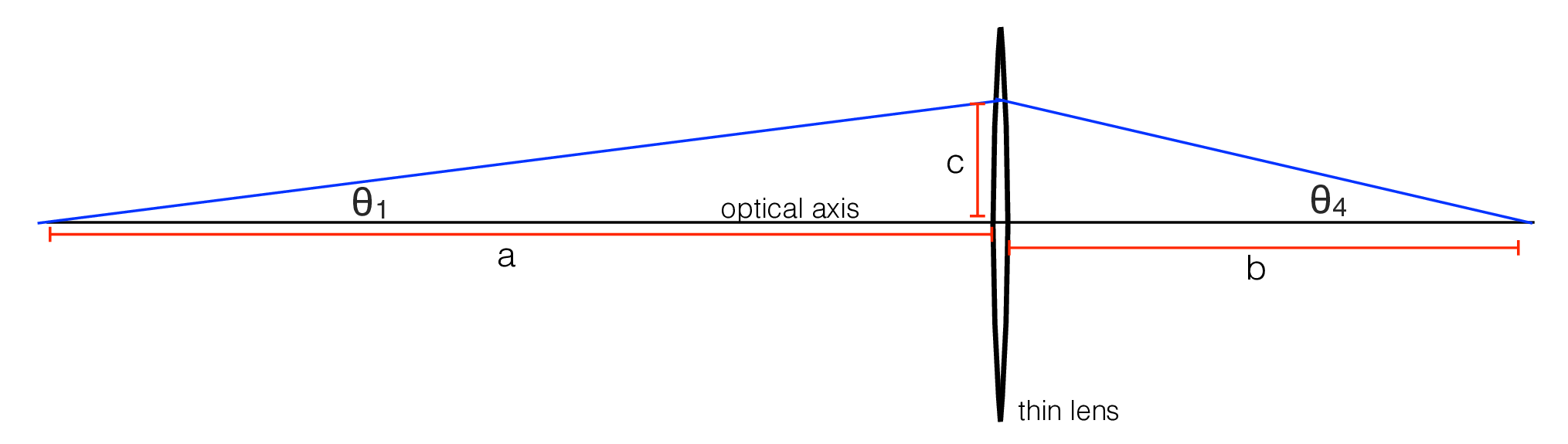
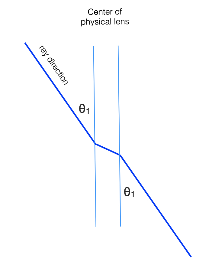
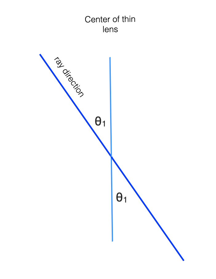
We make use of several approximations that commonly hold for imaging systems: the deviations in angle from the optical axes are very small (i.e., the paraxial approximation) and the lens is modeled to have negligible thickness compared with other distances along the optical axis (i.e., the thin lens approximation). Under those approximations, we can write simple expressions for the bending angles shown in a Figure 6.4 (b) a function of \(\theta_S\), the lens surface orientation at height \(c\). Those relations are summarized below in table Table 6.1.
The middle row of table Table 6.1 requires explanation. The light ray within the lens, depicted in Figure 6.4 (b), is not necessarily parallel to the optical axis. In general, it will be rotated by some angle \(\delta\) away from the optical axis, giving \(\theta_S = \theta_2 + \delta\), and, at the other lens surface, \(\theta_S = \theta_3 - \delta\). Adding those two equations removes \(\delta\) and gives the relation \(2 \theta_s = \theta_2 + \theta_3\)
| Angle | Description | Relation | Reason |
|---|---|---|---|
| \(\theta_1\) | Initial angle from optical axis | \(\theta_1 = c/a\) | Small angle approx. |
| \(\theta_2\) | Angle of refracted ray wrt front surface normal | \(n \theta_2 = \theta_1 + \theta_S\) | Snell’s law, small angle approx. |
| \(\theta_3\) | Angle of refracted ray wrt back surface normal | \(2 \theta_S = \theta_2 + \theta_3\) | Symmetry of lens, thin lens approx. |
| \(\theta_4 + \theta_S\) | Angle of ray exiting lens wrt back surface normal | \(n \theta_3 = \theta_4+\theta_S\) | Snell’s law, small angle approx. |
| \(\theta_4\) | Final angle from optical axis | \(\theta_4 = c/b\) | Small angle approx. |
If we start from the relation in table Table 6.1 for \(\theta_4\), and substitute for each angle using the relation in each line above, up through \(\theta_1 = c/a\), we can algebraically eliminate the angles \(\theta_1\) through \(\theta_4\) to find the condition on the lens surface angle, \(\theta_S\), as a function of the distance \(c\) from the optical axis, which allows for the desired focusing to occur. The result is as follows: \[\theta_S = \frac{c}{2(n-1)} \left( \frac{1}{a} + \frac{1}{b} \right) \tag{6.1}\]
This relationship creates the effect that every ray emanating at a small angle from point \(a\) will be focused to point \(b\). Equation 6.1 shows that the lens surface angle, \(\theta_S\), must deviate from flat in linear proportional to the distance \(c\) from the center of the lens.
To focus, the lens surface angle, \(\theta_S\), must be a linear function of the distance, \(c\), from the center of the lens.
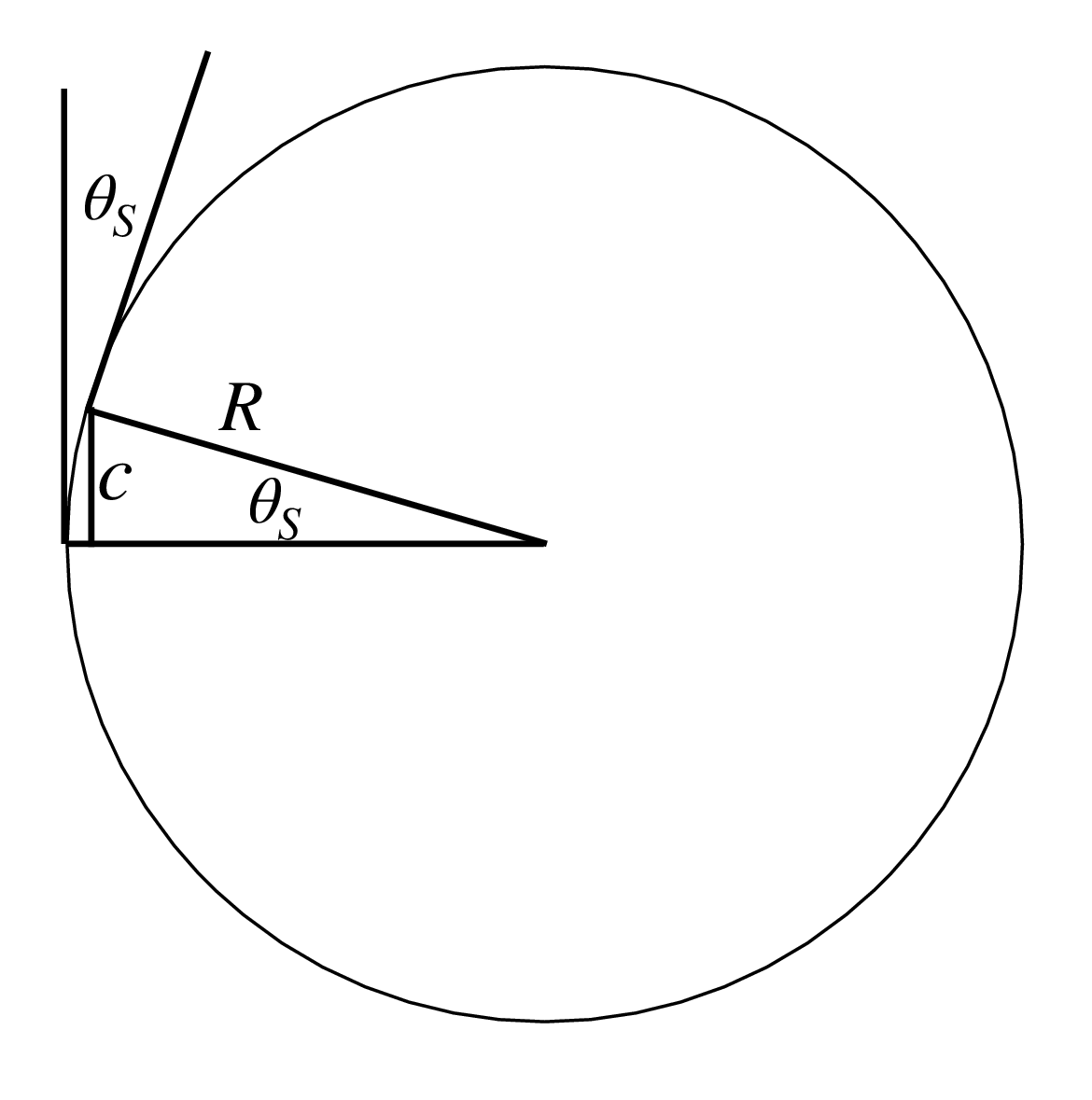
In the thin lens approximation, both parabolic and spherical shapes satisfy that constraint on the lens surface slope. For a spherical lens surface, such as Figure 6.5, curving according to a radius \(R\), we have \(\sin(\theta_S) = c/R\). For small angles \(\theta_S\), this reduces to \[\theta_S = \frac{c}{R}, \tag{6.2}\] where \(R\) is the radius of the sphere, which has the desired property that \(\theta_S \propto c\).
Substituting into the focusing condition, yields the Lensmaker’s Formula,
\[ \frac{1}{a} + \frac{1}{b} = \frac{1}{f}, \tag{6.3}\] where the lens focal length, \(f\) is defined to be
\[f = \frac{R}{2(n-1)}\]
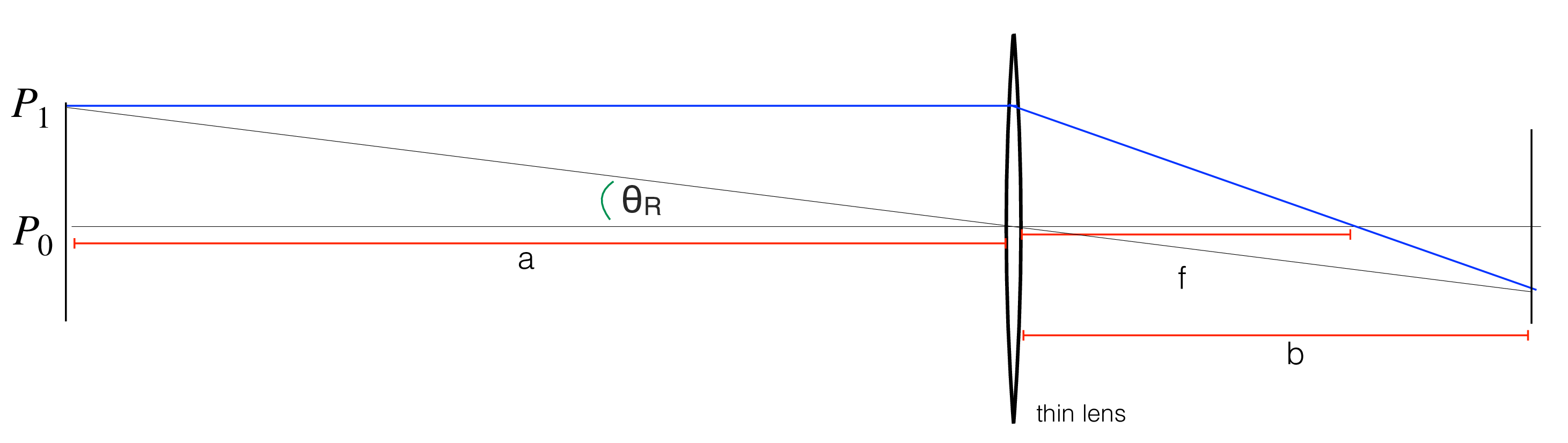
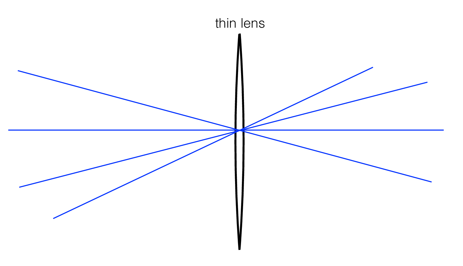
It is straightforward to show, by rotating the lens in Figure 6.4 (a) through an angle \(\theta_R\) in the above derivation, thus adding \(\theta_R\) to \(\theta_S\) in table Table 6.1, that the lensmaker’s equation also holds for light originating off the optical axis. Thus, under the paraxial and thin lens approximations, the lens focuses light from points on a plane onto points on a second plane, both perpendicular to the optical axis, as illustrated in Figure 6.6.
One can also generalize the equation for the case of a lens with different radii of curvature, \(R_1\) and \(R_2\) on the front and back faces of the lens. Defining the left and right surface angles \(\theta_{s_1}\) and \(\theta_{s_2}\), respectively, the middle row equation of table Table 6.1 becomes \(\theta_{s_1} + \theta_{s_2} = \theta_2 + \theta_3\). Then, the equation substitutions of Table Table 6.1, combined with \(\theta_{S_i} = c / R_i\), for \(i = 1\) and \(2\), lead to \[\frac{1}{f} = (n-1) \left( \frac{1}{R_1} + \frac{1}{R_2} \right)\]
Note that some texts (e.g., [1]) adopt a sign convention where the back surface of a lens is defined to have negative curvature.
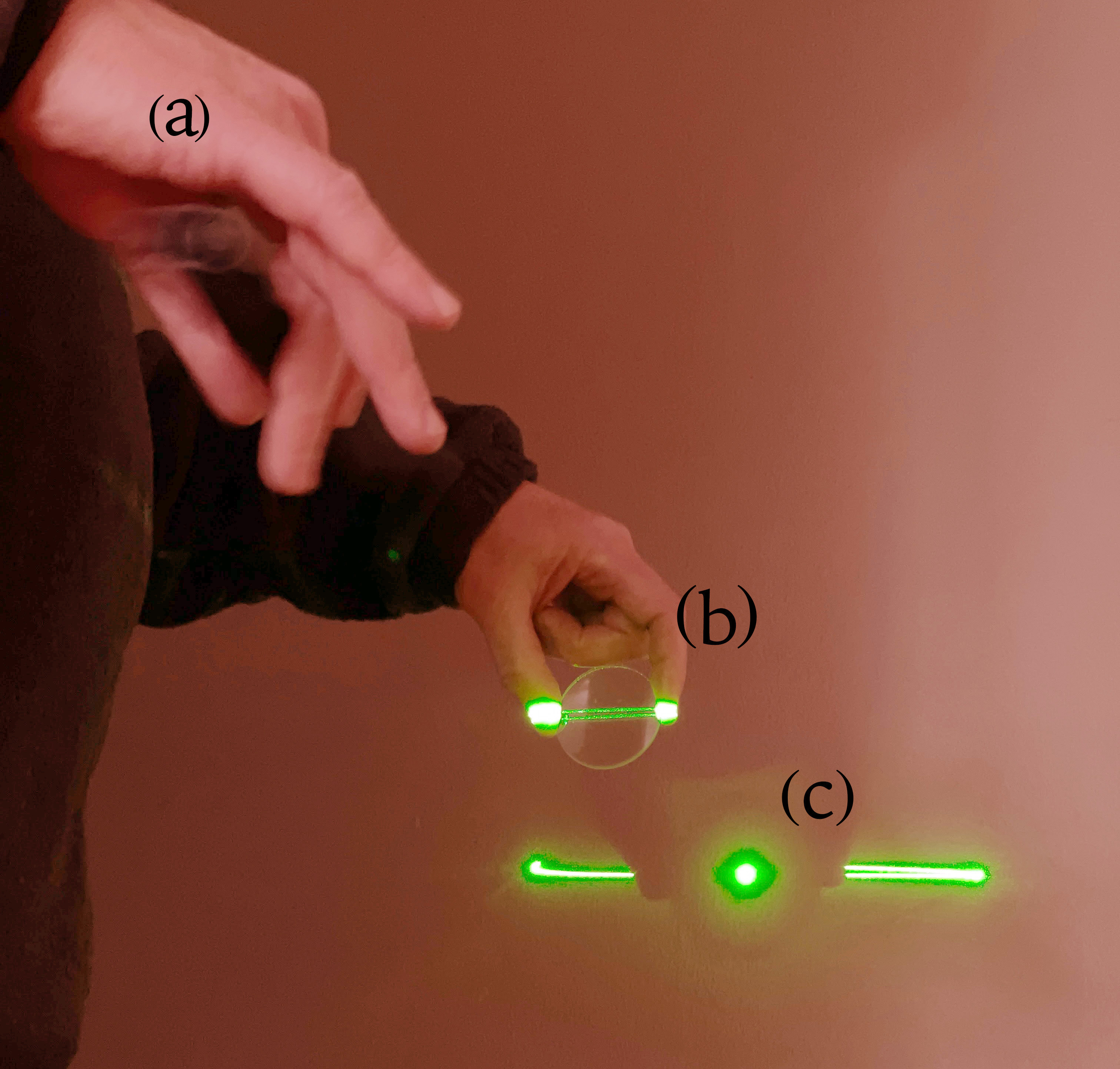
Figure 6.7 shows a demonstration of the focusing property for a thin lens. The hand, labeled (a), is flicking a laser pointer back and forth, sending light rays in many directions from a central point during the image exposure, as would a diffuse surface reflection. All the light rays that strike the lens, labeled (b), are focused to the same green spot, labeled (c), while the light rays passing outside the lens at (b) reveal their straight line trajectories on the wall at (c).
6.3 Imaging with Lenses
Armed with the lensmaker’s formula and the observation of Figure 6.8, we can analyze how rays travel through lenses in the approximation of geometrical optics. Light passing through the center of a thin lens, where the front and back surfaces are parallel, proceeds without bending. Thus a convex thin lens images as a pinhole camera does, creating a perspective projection.
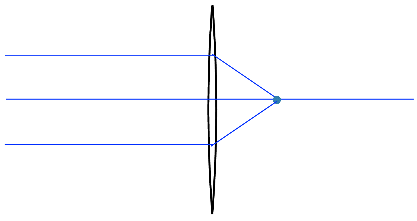
Two points on opposite sides of the lens at distances \(a\) and \(b\) from the lens that satisfy Equation 6.3 are known as conjugate points. Light from one conjugate point, traveling through the lens, focuses to the other conjugate point, and vice versa (see Figure 6.9). The rules for tracing light travel through a lens include the following:
Every ray passing through one conjugate point and passing through the lens then passes through the conjugate point. This is the fundamental focusing property of a lens.
Parallel rays entering the lens all focus to a point at distance \(f\) behind the lens, per Equation 6.3. In this case, one of the focal points is at infinity.
Any ray passing through the center of the thin lens proceeds in a straight line, as if through a pinhole at the center of the lens (see Figure 6.8). Thus, lenses, like pinholes, render the world in perspective projection.
Because focused rays render positions onto a plane as does a line passing through the center of the lens, then the magnification of a lens is simply \(a/b\), where \(a\) is the distance of an infocus object to the lens, and \(b\) is the distance from the lens to a sensor plane.
The above properties allow us to analyze the light paths through simple configurations of lenses.
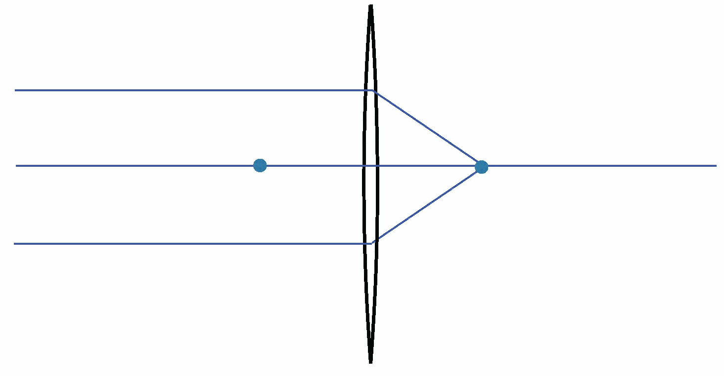
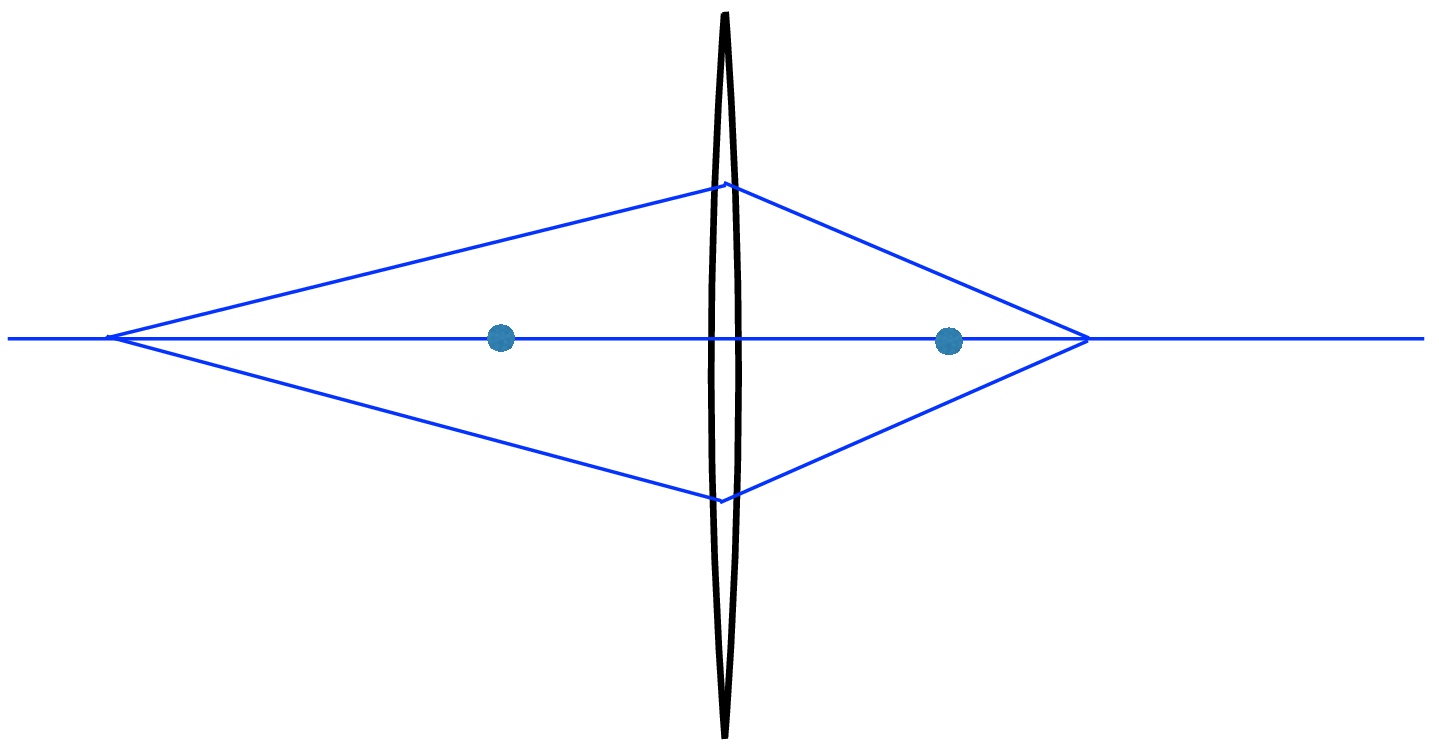
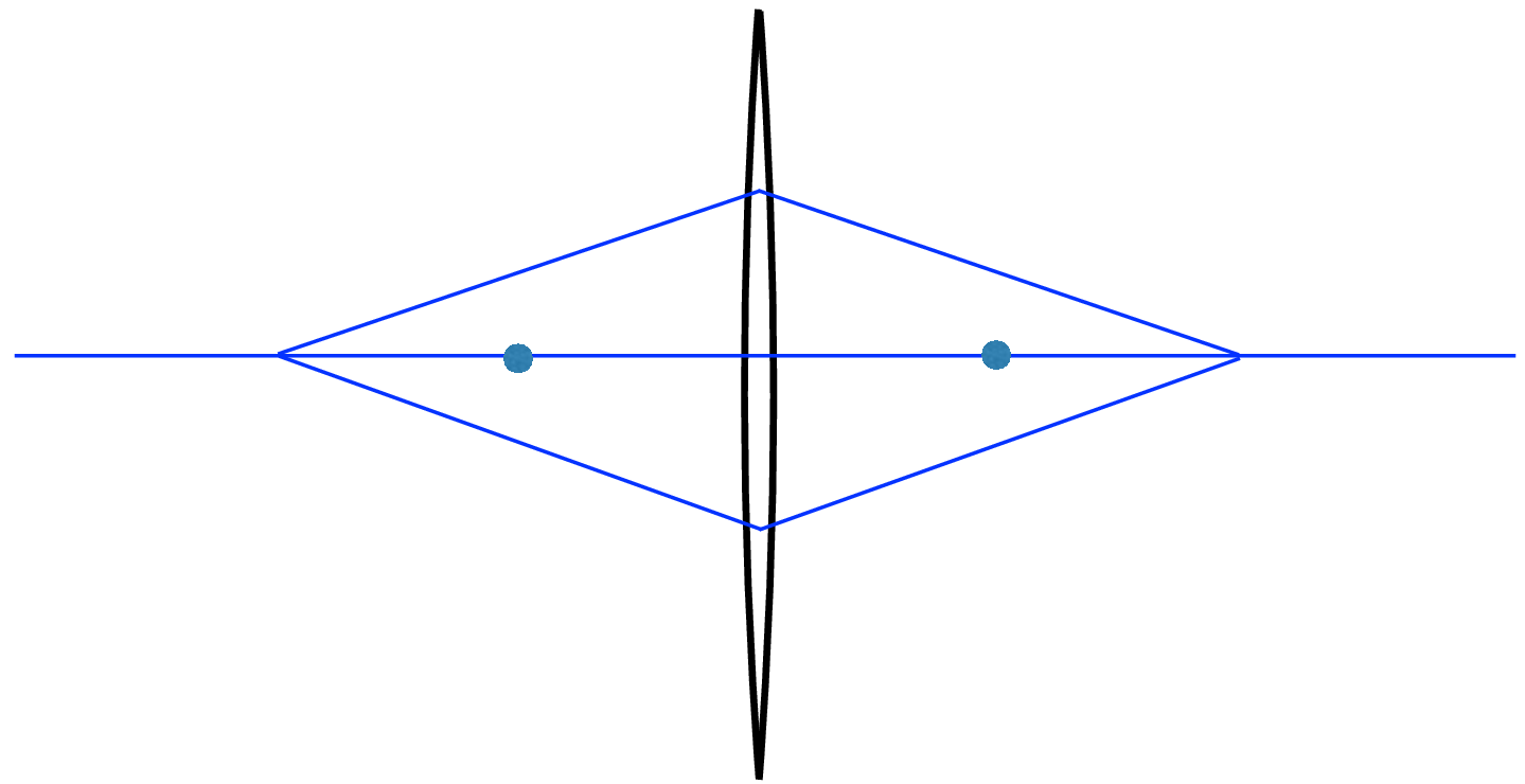
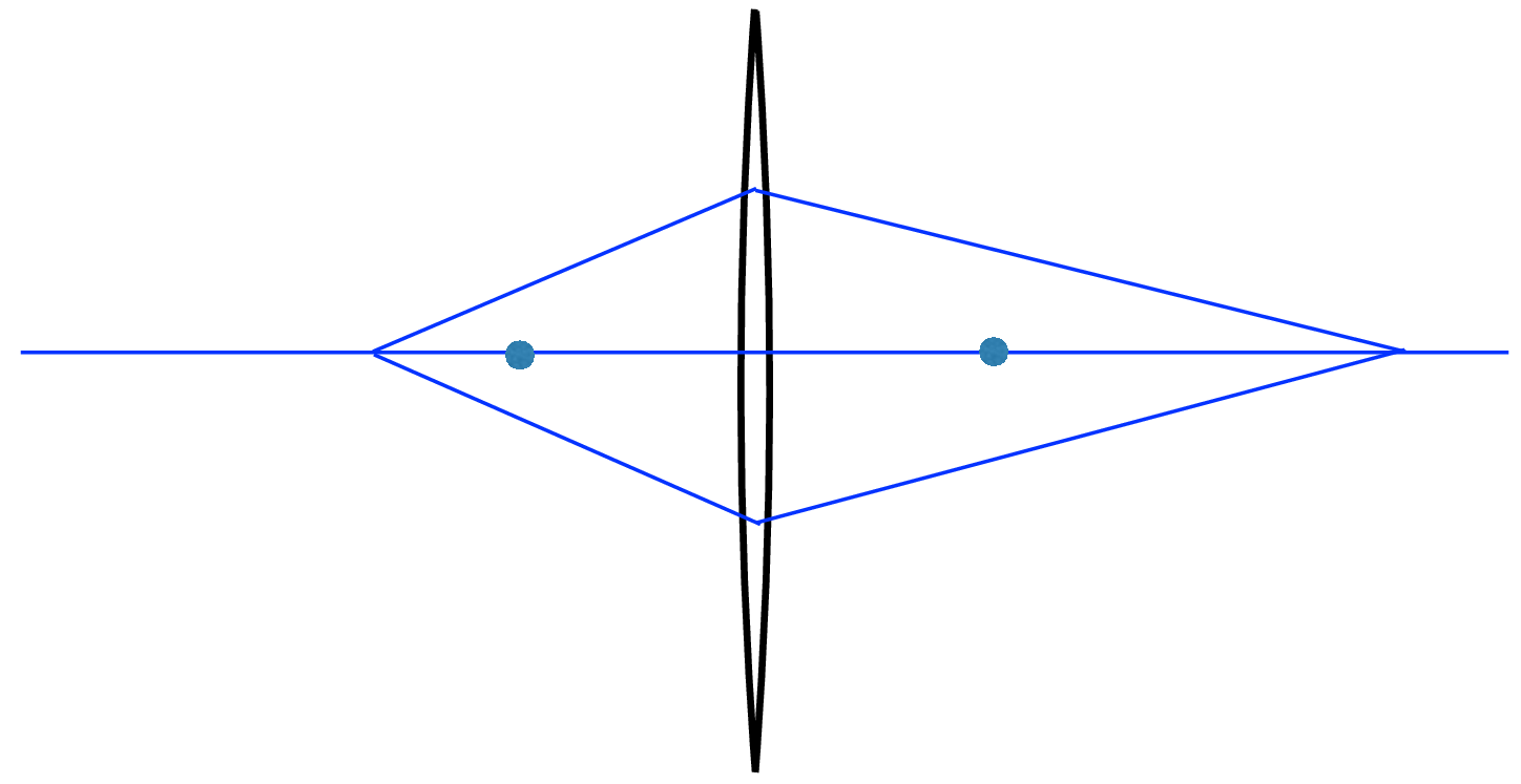
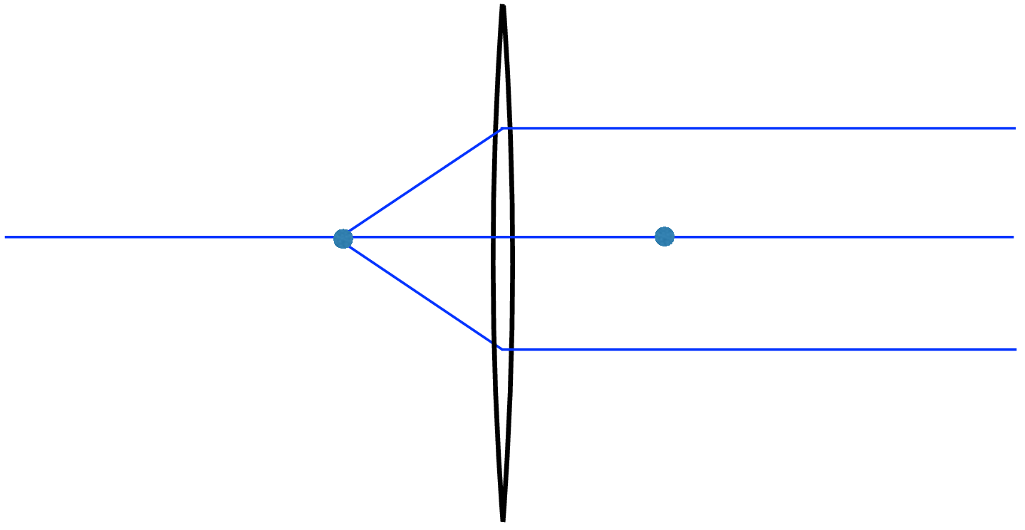
Referring to Figure 6.9, the two dots are at distance \(f\) from the lens. In Figure 6.9 (a), parallel rays from infinity focus at a distance f from the lens. Figure 6.9 (b) to Figure 6.9 (d) show that as a source of light rays moves closer to the lens, they focus further away on the other side, while Figure 6.9 (e) shows how rays emanating from a distance \(f\) from the lens are parallel after the lens, that is, they focus at infinity.
6.3.1 Depth of Field
Assume that the lens is part of a camera, focusing light from the world onto the camera’s sensor. If a plane outside of the camera, called the focal plane, and the camera’s sensor plane are at conjugate positions, then an object in the focal plane is focussed sharply onto the sensor plane. All rays from a point on the object’s surface will come into focus at a point in the sensor plane. This will image a point in the focal plane to a circle of confusion at the sensor plane, as illustrated in Figure 6.10.
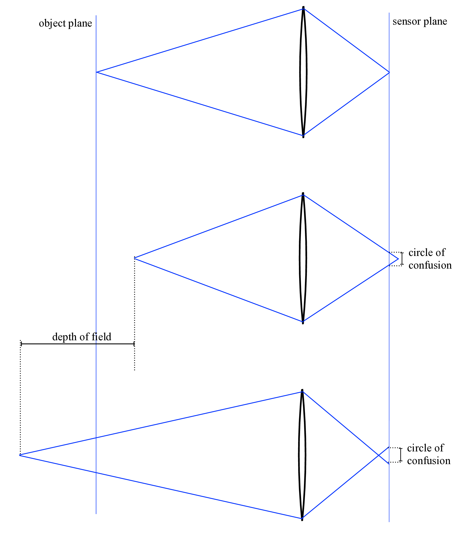
Objects closer or further from the focal plane will come into focus behind or in front of the sensor plane, respectively, resulting in a blur circle at the sensor plane, as illustrated in figures Figure 6.10 and Figure 6.11.
The region around the plane of focus that results in a blur at the sensor plane that is smaller than some tolerance is called the depth of field. We can calculate the depth of field from geometric considerations. This derivation follows that of Marc Levoy [2].
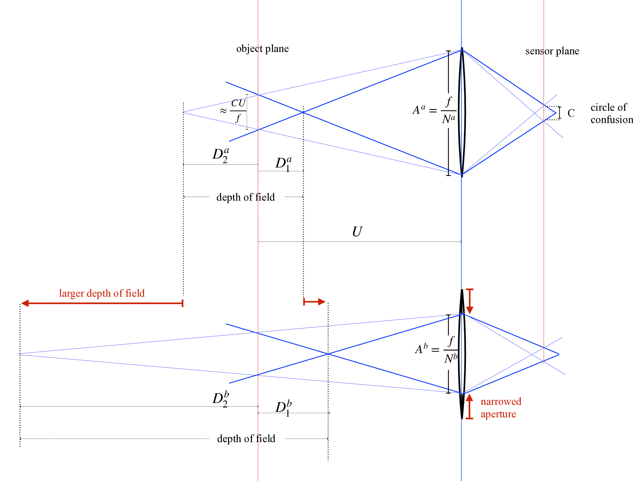
A camera’s f-number, written \(N\), is the ratio of the focal length of the lens divided by the diameter of the lens that light passes through, called the aperture, A: \(N = f/A\). Let the diameter of the circle of confusion be \(C\). If the distance, \(U\), of the focal plane to the camera is much larger than the focal length of the lens (\(U >> f\)) then the diameter of the focal plane that is imaged onto the circle of confusion is \(C\) times the magnification of the imaging system, or approximately \(C U/f\), again, for \(U >> f\). Referring to the top of Figure 6.10, by similar triangles, we have \[\frac{D_1 f}{C U} = \frac{U - D_1}{\frac{f}{N}}\] Also by similar triangles, we have \[\frac{D_2 f}{C U} = \frac{D_2+U}{\frac{f}{N}} \] Defining the depth of field, \(D\), to be \(D = D_1 + D_2\), and combining terms, we have \[D = \frac{2 N C U^2 f^2}{f^4 - N^2 C^2 U^2}\]
When the circle of confusion, \(C\), is much smaller than the lens aperture, \(f/N\), then the term \(N^2 C^2 D^2\) can be ignored relative to \(f^4\), and we have \[D \approx \frac{2 N C U^2}{f^2}\] Note that for smaller camera f-numbers, \(N\) (larger apertures), the depth of field decreases in proportion. This effect can be seen in the bottom of Figure 6.11, and in Figure 6.12.
 {(a) f/2.0}
 {(b) f/4.0}
 {(c) f/8.0}
6.3.2 Concave Lenses
The lens we designed in Section 6.2 was convex. Also of interest are concave lenses, with the lens surface curve bowing inward toward the center of the lens. For example, consider the concave lens with the surface orientation, \(\theta_{Sx} = -\theta_S\) in Equation 6.3. By the reflection symmetry of the lens surface angles, parallel rays entering a concave lens will be bent away from the lens center by the same amount it would be bent toward the center axis for a convex lens of the same lens radii of curvature. This leads to a concave lens bringing parallel rays to a virtual focus, a point from which the diverging rays leaving the lens appear to be emanating. This is illustrated in Figure 6.13 (b) on-axis, and Figure 6.13 (c) for off-axis parallel rays.
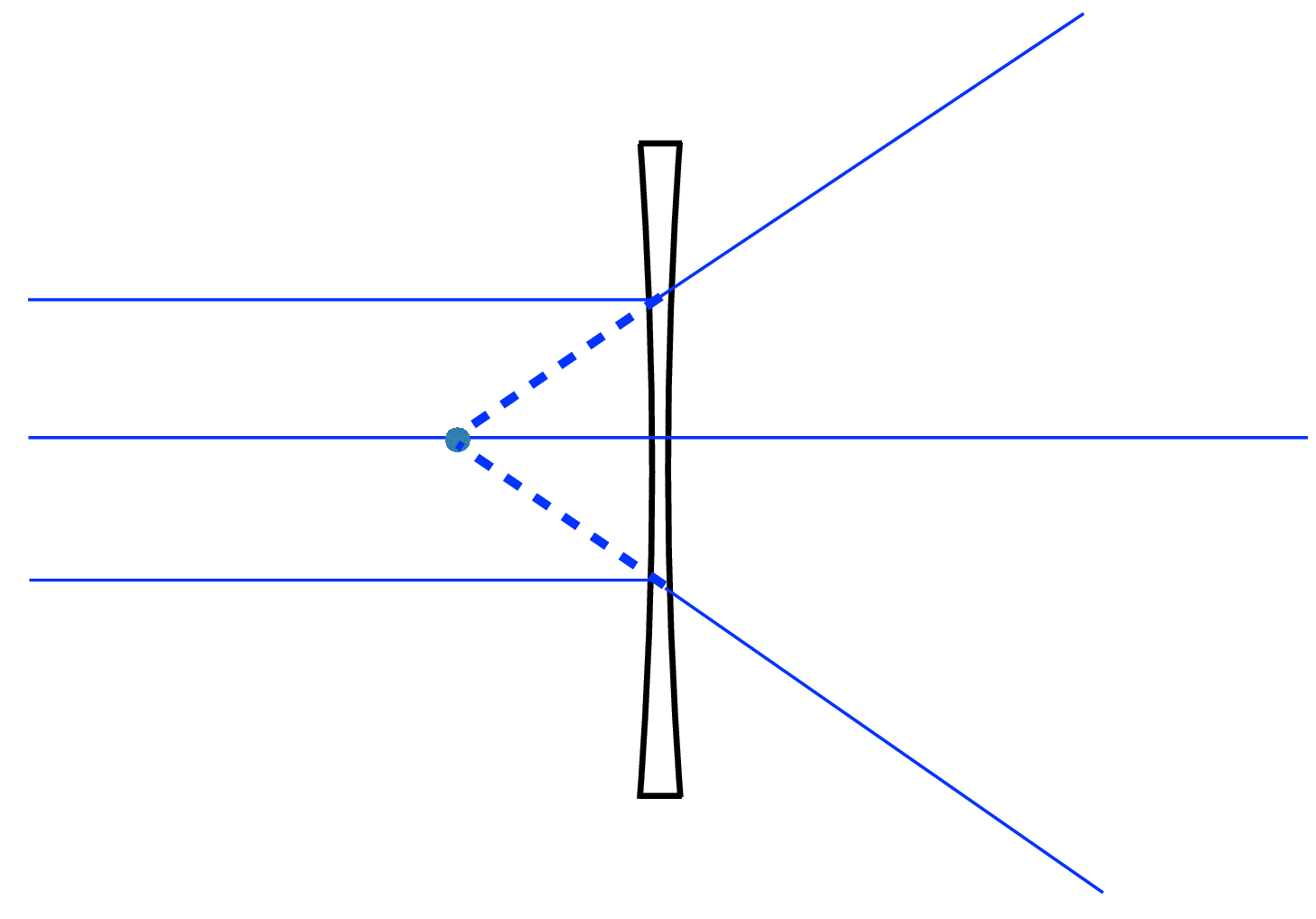
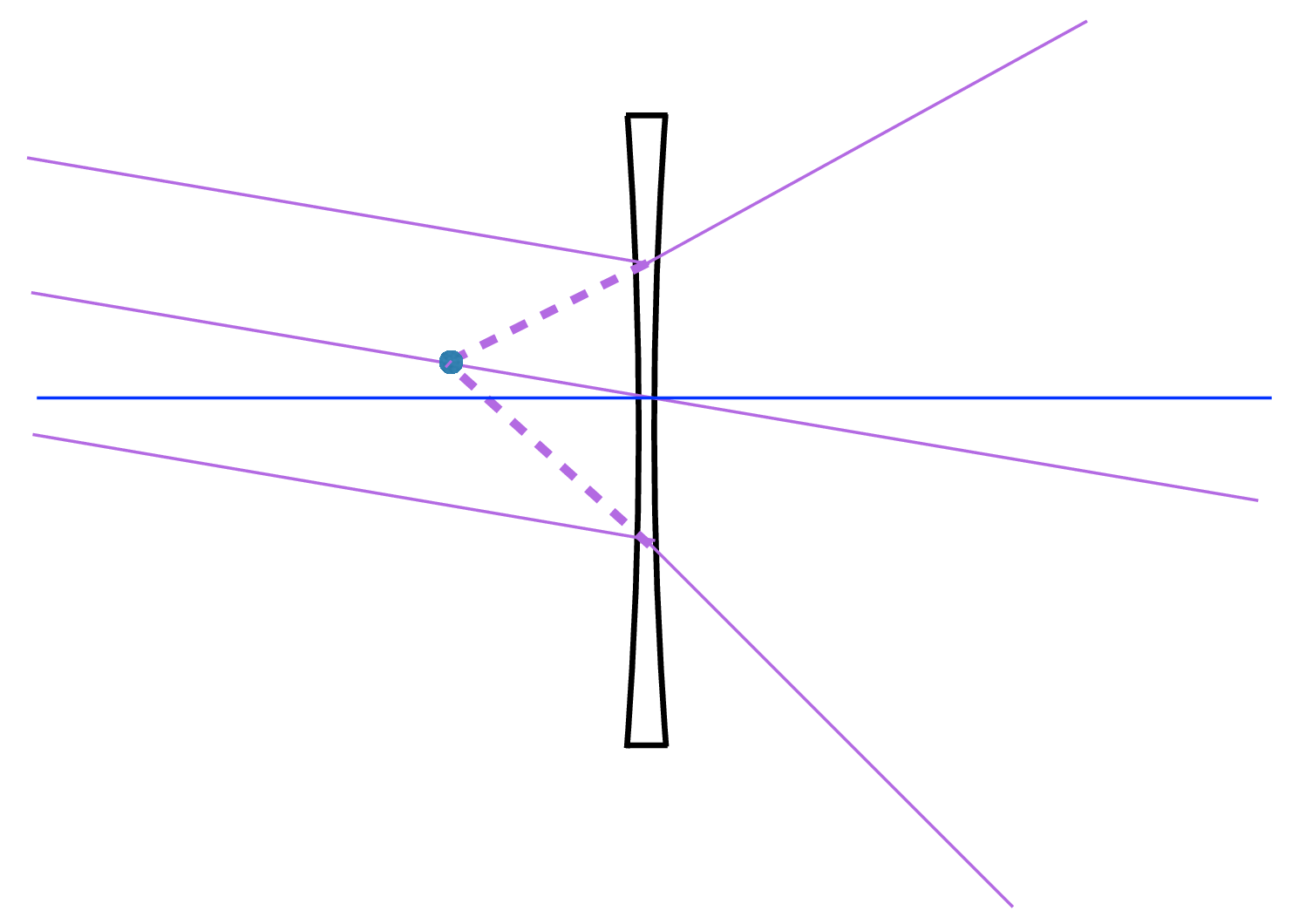
The mathematics of the ray bending is similar to that for convex lenses, except the focal length of concave lenses has a negative value, illustrated in Figure 6.13. The focus point for a set of parallel rays entering a concave lens from the left is also on the left side of the lens. It is a virtual focal point, and from the right side of the lens, the emanating rays appear to be originating from the point at distance \(-f\) to the left of the lens.
6.3.3 Lenses in a Telescope
The properties of convex and concave lenses can be used to make a telescope, as Galileo did in the early 1600s [3]. We can see how the telescope magnifies the size of objects from geometric considerations. As shown in Figure 6.14 (a), we position a convex lens, lens 1, with a long focal length, \(f_1\), and a concave lens, lens 2, with a shorter focal length, \(f_2\), such that each are \(f_1\) and \(f_2\) away from some common point, respectively. Under those conditions, the configurations of figures Figure 6.13 (a) and Figure 6.13 (b) will cause parallel rays from a distant object entering lens 1 to become a compressed set of parallel rays leaving lens 2. Referring to Figure 6.14 (b), an angular deviation of the input rays of \(\delta_i\) will become an angular deviation, exiting the convex lens of \(\delta_o\).

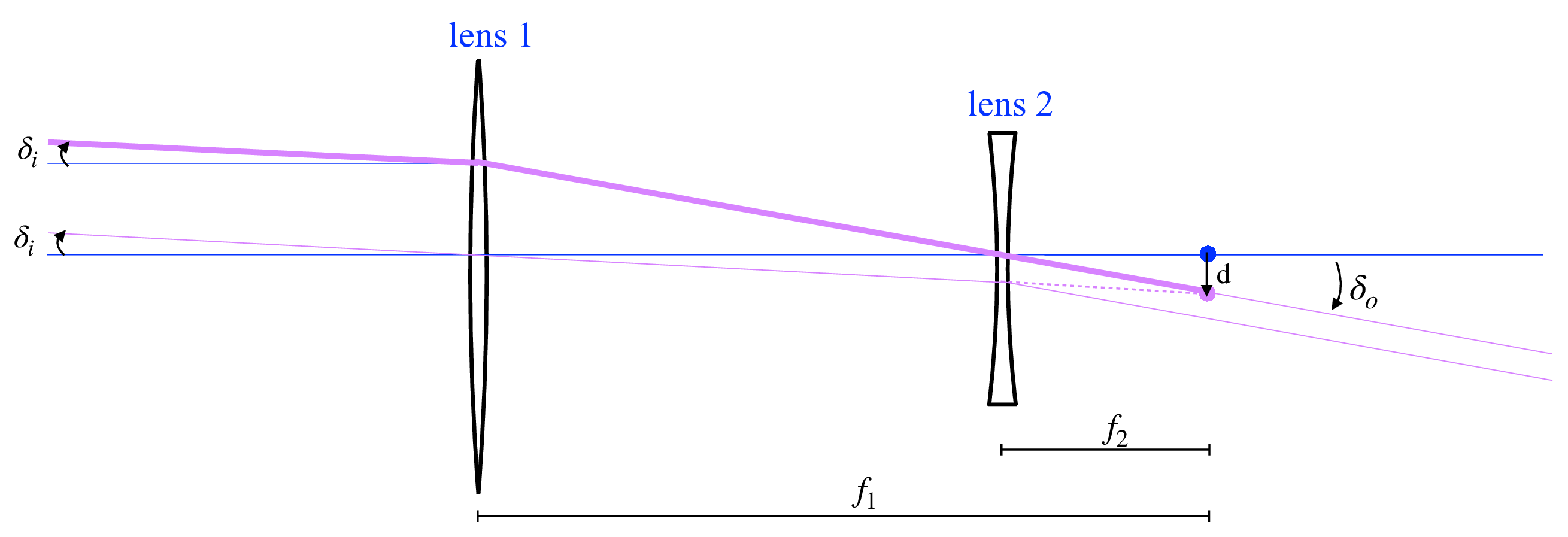
By property 3 of Section 6.3, and the small angle approximation, we have \(\delta_i f_1 = d\), because the point \(p\) is a distance \(f_1\) from lens 1. Similarly, we have \(\delta_o f_2 = d\). Substituting for \(d\) gives \[M = \frac{\delta_o}{\delta_i} = \frac{f_1}{f_2},\] where we have defined the telescope magnification, \(M\), to be the amplification of the parallel ray bending angles.
Figure 6.15 shows a homemade telescope, inspired by Galileo’s. The tube is a 2 in. cardboard mailing tube, with a second tube inserted within it to allow the interlens distance to be adjusted for focusing. The convex lens at the front of the telescope has a focal length of 50 cm, and the convex lens eyepiece has a focal length of 18 mm, giving a magnification of 27. This is comparable to the 30x magnification of Galileo’s telescope.
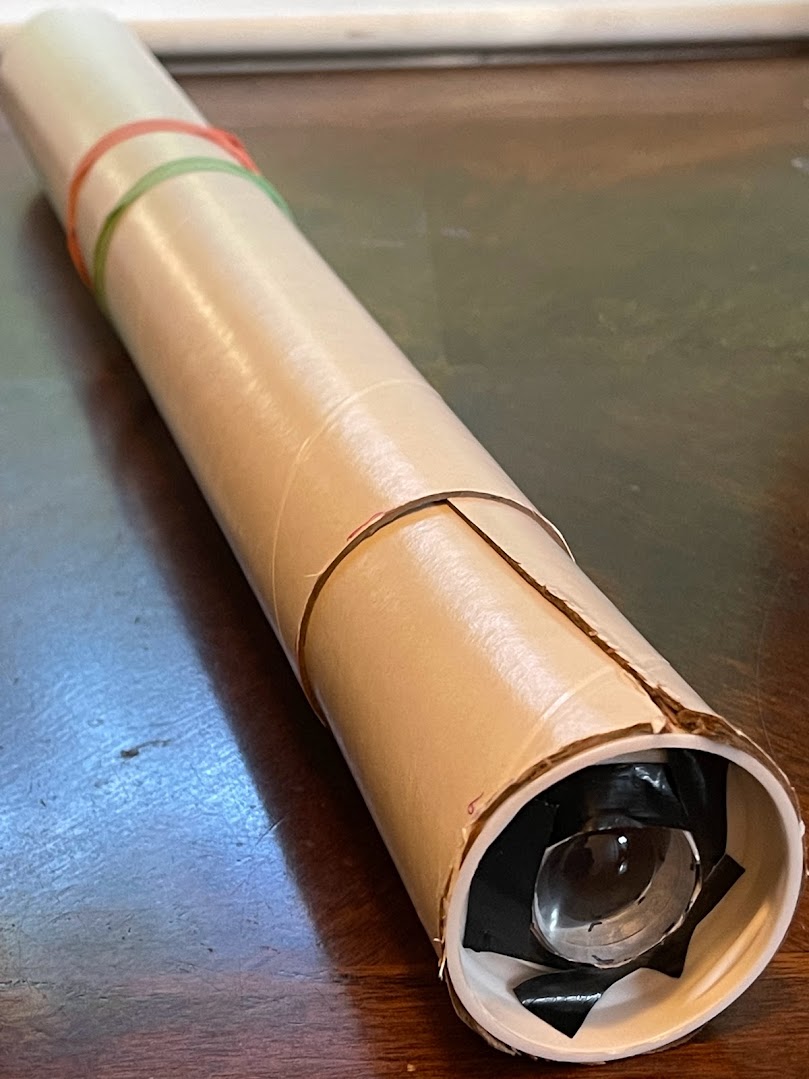
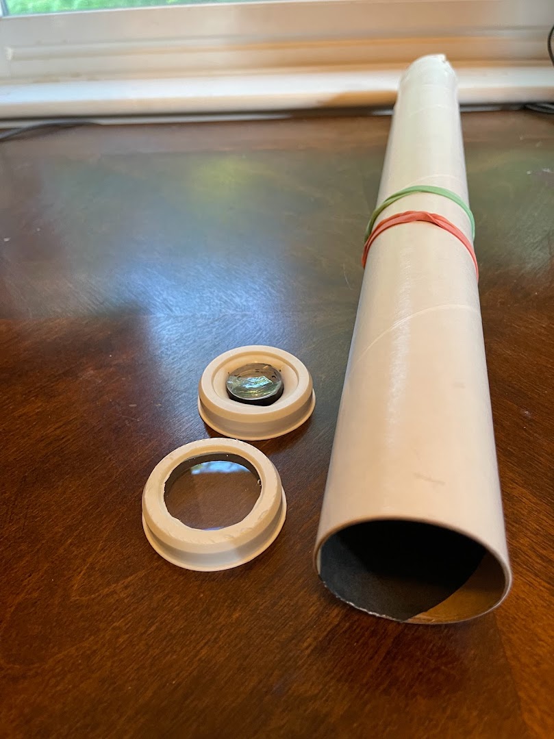
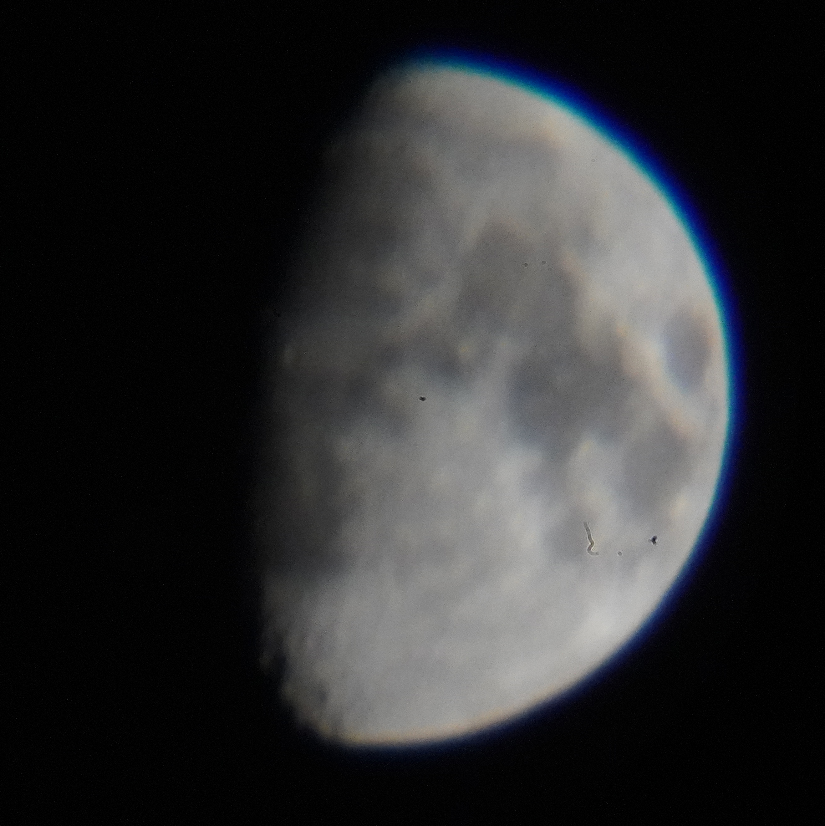
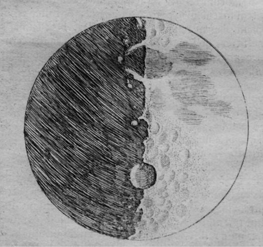
Figure 6.16 compares images made from this homemade telescope with drawings Galileo made of what he saw through his telescope. He discovered that our moon had mountains and craters, and was thus not a perfect sphere, as some had thought. While he could not resolve the rings of Saturn, he could see that there was something different about its shape. These can all be seen from just two lenses within a tube!
With his telescope, Galileo discovered four of the moons of Jupiter. He called them the Medician Stars, in honor of the brothers of the Medici family, who were prospective patrons.
6.4 Concluding Remarks
Pinhole cameras can allow more light to enter the camera aperture only at the expense of image sharpness. Lenses overcome that tradeoff by focusing all the rays passing through the lens from a point on a surface to a single position on the sensor plane, creating an image that is both sharp and bright.
Using small-angle and thin-lens approximations, we designed a lens surface to have that focusing property, showing that the lens must have a parabolic or spherical shape.
Geometric considerations allow depth-of-field calculations, as well as the design of a simple telescope.