45 Radiance Fields
45.1 Introduction
In this chapter we will come full circle. Starting from the Greek’s model of optics (Chapter 1) that postulated that light is emitted by the eyes and travels in straight lines, touching objects in order to produce the sensation of sight (extramission theory), radiance fields will use that analogy to model scenes from multiple images. Here, geometry-based vision and machine learning will meet.
Before diving into radiance fields, we will review Adelson and Bergen’s plenoptic function; a radiance field can be considered as a way to represent a portion of the plenoptic function.
45.1.1 The Plenoptic Function
We first discussed the plenoptic function when we introduced the challenge of vision in Chapter 1.
As stated in the work by Adelson and Bergen [1], the plenoptic function tries to answer the following question: “We begin by asking what can potentially be seen. What information about the world is contained in the light filling a region of space?”
Given a scene, the plenoptic function is a full description of all the light rays that travel across the space (Figure 45.1). The plenoptic function tells us the light intensity of a light ray passing through the three-dimensional (3D) point \((X, Y, Z)\) from the direction given by the angles \((\psi, \phi)\), with wavelength \(\lambda\), at time \(t\): \[L(X, Y, Z, \psi, \phi, \lambda, t)\] In this chapter wewill ignore time and we will only use three color channels instead of the continuous wavelength. We can represent the plenoptic function with the parametric form \(L_{\theta}\) where the parameters \(\theta\) have to be adapted to represent each scene.
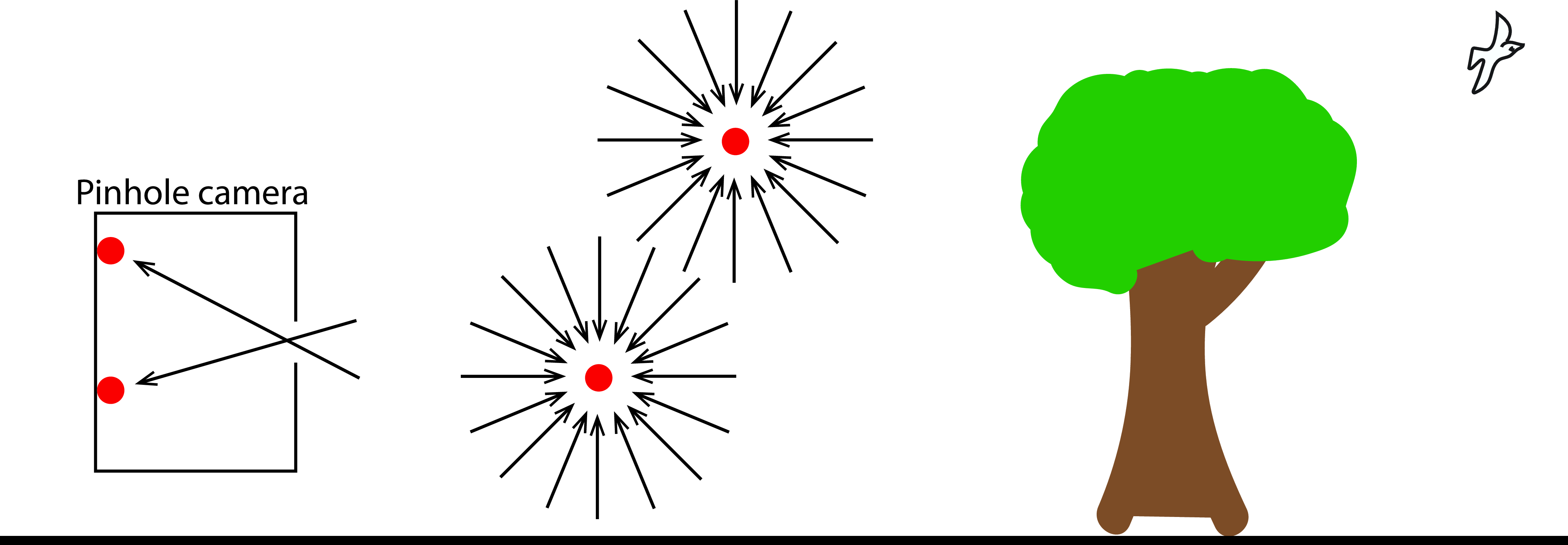
An image gets formed by summing all the light rays that reach each sensor on the camera (that is, we sum over a section of the plenoptic function). Figure 45.1 shows an illustration of the plenoptic function at four points, two of them are inside a pinhole camera and are used to form an image of what is outside. The plenoptic function inside the pinhole camera has most of the values set to zero and only specific directions at each location have non-zero values.
In Chapter 1 we discarded the plenoptic function by simply saying, “Although recovering the entire plenoptic function would have many applications, fortunately, the goal of vision is not to recover this function.” But we did not really give any argument as to why simplifying the goal of vision was a good idea. What if we now we change our minds and decide that one useful goal of vision is to actually recover that function entirely? Can it be done? How?
If we had access to the plenoptic function of a scene, we would be able to render images from all possible viewpoints within that scene. One attempt at this is the [2] which extracts a subset of the plenoptic function from a large set of images showing different viewpoints of an object. Another approach, [3], also uses many images to get a continuous representation of the field of light in order to be able to render new viewpoints (with some restrictions). This chapter will mostly focus on a third approach to modeling portions of the plenoptic function, where we model a scene with a radiance field that assigns a color and volumetric density to each point in 3D space.
45.2 What is a Radiance Field?
A radiance field is a representation of part of the plenoptic function, based on the idea that the optical content of a scene can be modeled as a cloud of colorful particles with different levels of transparency. Such a representation can be rendered into images using volume rendering, which we will learn about in Section 45.4. Radiance fields come in a variety of configurations but we will stick with the definition from Mildenhall et al. [4], which popularized this representation. We will presently define a radiance field \(L\) as a mapping from the coordinates in a scene to color and density (i.e. transparency) values of the scene content at those coordinates. The coordinates can be two-dimensional (2D) (\(X,Y\)) for a 2D world, or 3D (\(X,Y,Z\)) for a 3D world. They may also contain the angular dimensions (\(\psi\) and \(\phi\)) that represent the viewing angle from which we are looking at the scene. Representing color using \(r,g,b\) values, and representing density with a scalar \(\sigma\), a radiance field is therefore a function:
\[\begin{aligned} L: X,Y,Z,\psi,\phi \rightarrow r,g,b,\sigma \quad\quad\triangleleft \quad\text{radiance field} \end{aligned}\]
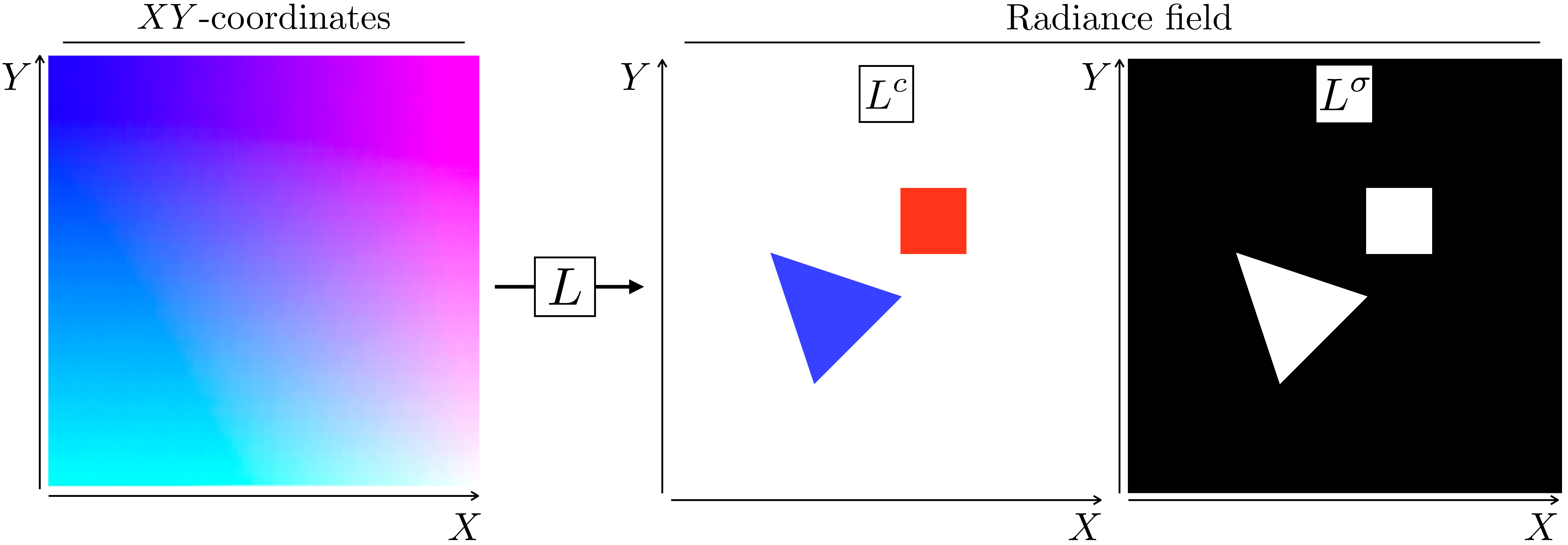
The angular coordinates \(\psi\) and \(\phi\) allow that an object’s color be different depending on the angle we look at it, which is the case for shiny surfaces and many other materials. We will use the terms \(L^c\) and \(L^\sigma\) to denote the subcomponents of \(L\) that output color and density values respectively: \[\begin{aligned} L^c&: X,Y,Z,\psi,\phi \rightarrow r,g,b\\ L^{\sigma}&: X,Y,Z,\psi,\phi \rightarrow\sigma \end{aligned}\]
45.2.1 A Running Example: Seeing in Flatland
For simplicity, we will study radiance fields for a 2D world. Radiance fields in 3D are the same thing just with one more dimension. This 2D world is like the one in Flatland, which is a book by Edwin Abbott [5] where the characters are triangles, squares, and other simple shapes that inhabit a 2D plane. Here is what their world looks like (Figure 45.2):
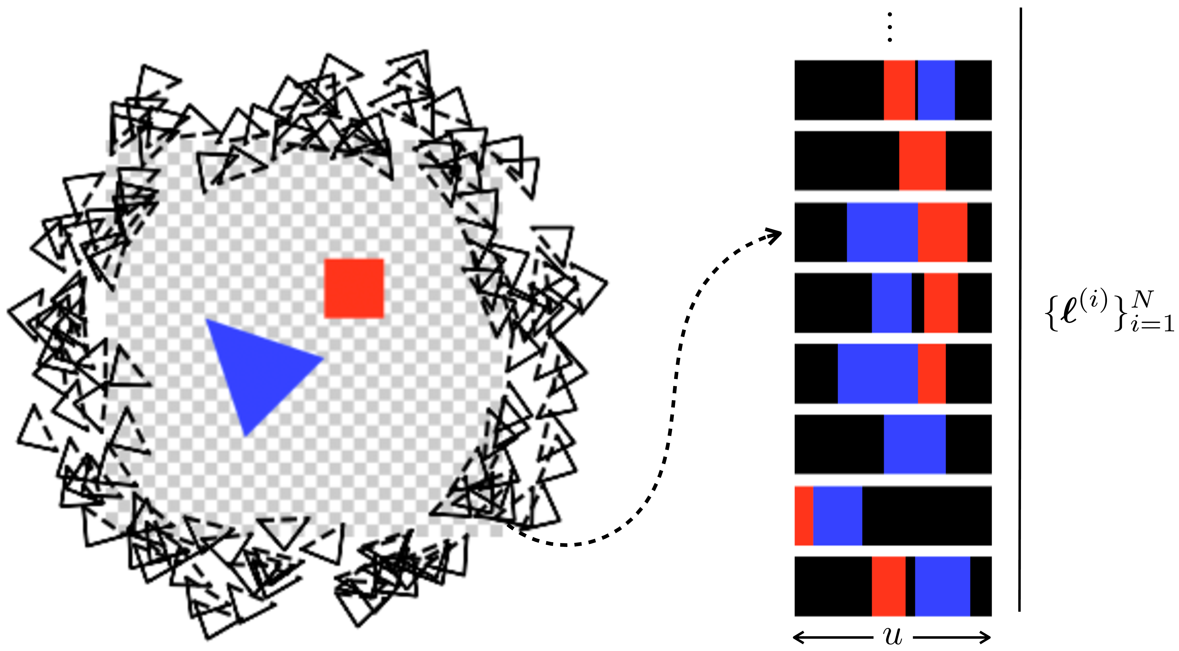
On the left is a top-down image of the world, but inhabitants of Flatland cannot see this. Instead they see the images on the right, which are one-dimensional (1D) renderings of the 2D world. The circle of black triangles on the left are cameras that result in the 1D photos seen on the right. These show what our Flatland citizens would see if they look at the scene from different angles.
A radiance field for this scene is given in Figure 45.3. This figure shows how each possible input coordinate \((X,Y)\) gets mapped to a corresponding output color \(L^c\) and density \(L^{\sigma}\).
45.2.2 Aside: Representing Scenes with Fields
Radiance fields are an example of vector fields, which are functions that assign a vector to each position in space. For example, we might have a vector field \(f: X, Y, Z \rightarrow v_1, v_2\), where \(X\), \(Y\) and \(Z\) are coordinates and \(v_1\) and \(v_2\) are some values. Let’s take a moment to consider field-based representations more broadly, since they turn out to be a very important way of representing scenes. Essentially, fields are a way to represent functions that vary over space, and fields appear all over the place in this book. For example, every image is a field: it is a mapping from pixel coordinates to color values. The images we usually deal with in computer vision are discrete fields (the input coordinates are discrete-valued) but in this chapter we will instead deal with continuous fields (the input coordinates are continuous-valued). Unlike regular images, fields can also be more than two-dimensional and can even be defined over non-Euclidean geometries like the surface of a sphere. Because they are such a general-purpose object, fields are used as a scene representation in many contexts. Some examples are the following:
Pixel images, \(f: x, y \rightarrow r, g, b\), are fields with the property that the input domain is discrete, or, equivalently, the field is piecewise constant over little squares that tile the space.
Voxel fields, \(f: X,Y,Z \rightarrow \mathbf{v}\) are discrete fields that can represent values \(\mathbf{v}\) like spatial occupancy, flux, or color in a volume. They are like 3D pixels. Like pixels, they have the special property that they are piecewise constant over cubes the size of their resolution.
Optical flow fields, \(f: x, y, t \rightarrow u, v\), measure motion in a video in terms of how scene content flows across the image plane. We encountered these fields in Chapter 47.
Signed distance functions (SDFs) [6], \(f: X,Y,Z \rightarrow d\), represent the distance to the closest surface to point \([X,Y,Z]^\mathsf{T}\). This is a useful representation of geometry.
Notation reminder: we use capital letters for world coordinates and lowercase letters for image coordinates.
As you read this chapter, keep in mind these other kinds of fields, and think about how the methods you learn next could be used to model other kinds of fields as well.
45.3 Representing Radiance Fields With Parameterized Functions
Continuous fields are powerful because they have infinite resolution. But this means that we can’t represent a continuous field explicitly; we cannot record the value at all infinite possible positions. Instead we may use parameterized functions to represent continuous fields. These functions take as input any continuous position and tell us the value of the field at that location. Sometimes this is called an implicit representation of the field, since we don’t explicitly store the values of the field at all coordinates. Instead we just record a finite set of parameters of a function that can tell us the value of the field at any coordinate. Recall that we learned about implicit image representations in Section 38.6.
Implicit representations are also used in variational autoencoders (VAEs) where we represent an infinite set (an infinite mixture of Gaussians) via a parameterized function from a continuous input domain (see ). You can consider a VAE to be a continuous field mapping from latent variables to images!
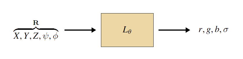
There are many different parameterized functions \(L_{\theta}\) that could represent our target radiance field \(L\). We could use a neural net (e.g., [4]), or a mixture of Gaussians (e.g., [7]), or any number of other function approximators. The important property we seek is that the field \(L_{\theta}\) is a differentiable function of the parameters \(\theta\), hence we can use gradient-based optimization to find a setting of the parameters that yields a desirable field (we will use this property when we fit a radiance field to images). Whatever function family we use, it will take as input coordinates and produce colors and densities as output (Figure 45.4). Because we will use differentiable functions for this, we can think of it just like a module in a differentiable computation graph (Figure 45.4). Later we will put together multiple such modules and use backpropagation to optimize the whole system to fit the field to a set of images.
45.3.1 Neural Radiance Fields (NeRFs)
We will focus our attention on one very popular way of parameterizing \(L_{\theta}\): Neural radiance fields (NeRFs) [4]. NeRFs model the radiance field \(L\) with a neural network \(L_{\theta}\). The neural network architecture in the original NeRF is a multilayer perceptron (MLP), but other architectures could be used as well. For the MLP formulation, evaluating the color-density at a single coordinate corresponds to a single forward pass through an MLP.
Often, however, we want to evaluate the color-density at multiple coordinate locations. To create an explicit representation of the field’s values at a grid of coordinates, we can query the field on this grid. In this usage, the NeRF \(L_{\theta}\) looks like a convolutional neural network (CNN) with 1x1 filters, as this is the architecture that results from applying an MLP to each position in a grid of inputs. We show this usage below, in Figure 45.5.
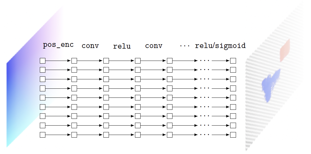
As in the original NeRF [4], the output layer is \(\texttt{relu}\) for producing \(\sigma\) (which needs to be nonnegative) and \(\texttt{sigmoid}\) for producing \(r,g,b\) values (which fall in the range \([0,1]\)).
NeRF also includes a positional encoding layer to transform the raw coordinates into a Fourier representation. In fact, we use the same positional encoding scheme as is used in transformers (see Section 26.11). Figure 45.6 shows how this scheme translates the \(XY\)-coordinate field of Flatland to positional encodings:
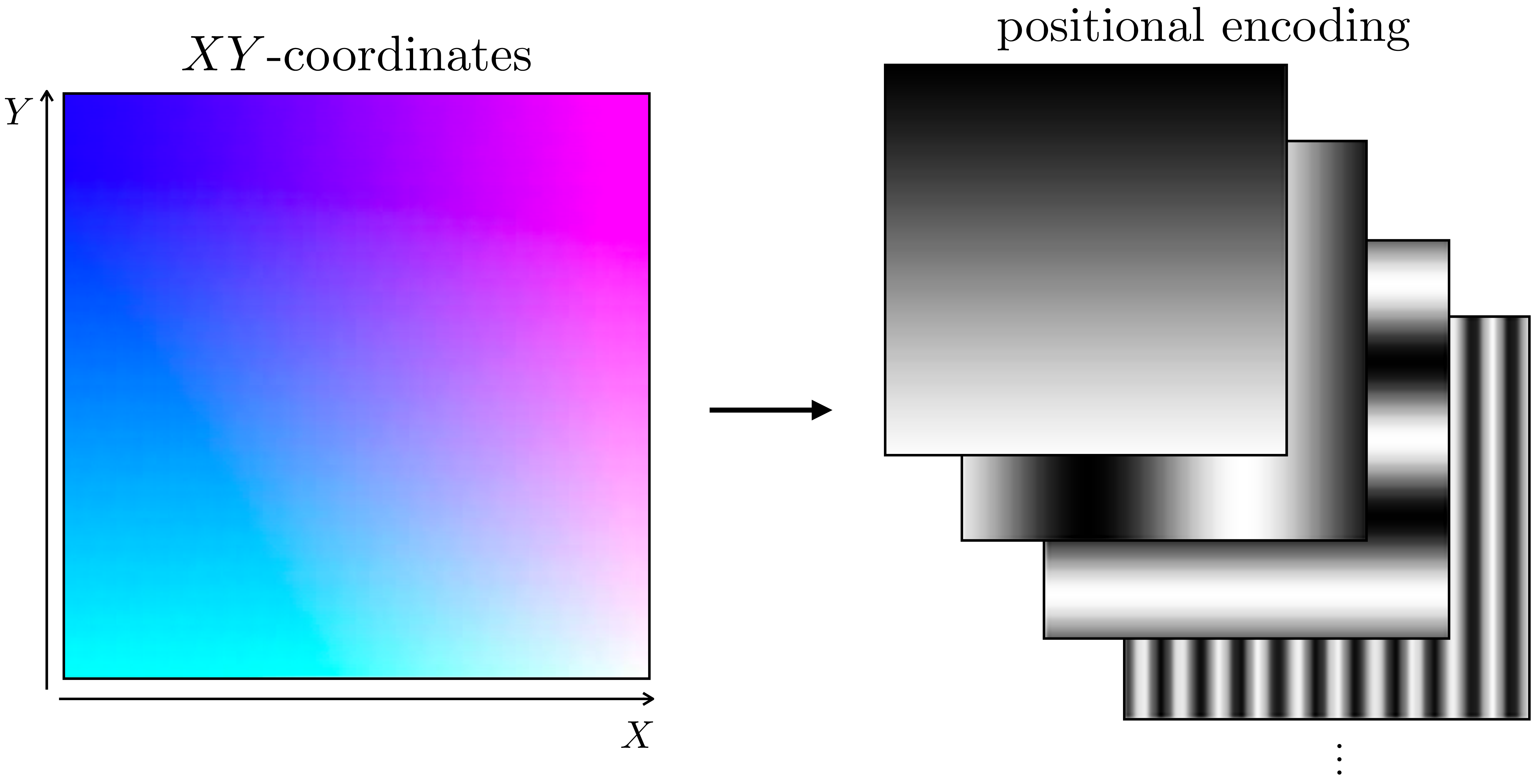
Fourier positional encodings are very effective for NeRFs because they help the network to model high frequencies variations, which are abundant in radiance fields [8]. Why do such encodings help model high frequencies? Essentially, in regular Cartesian coordinates, the location \((0,0)\) is much closer to \((1,1)\) than it is to \((100,100)\), but this isn’t necessarily the case with Fourier positional codes. Because of this, with Cartesian coordinates as inputs, an MLP will be biased to assign similar values to \((0,0)\) and \((1,1)\) and different values to \((0,0)\) and \((100,100)\). Conversely, with Fourier positional codes as input, this bias will be reduced. This makes it so the MLP, taking Fourier positional codes as input, has an easier time fitting high frequency functions that change in value rapidly, as in the case of assigning very different output values to the locations \((0,0)\) and \((1,1)\). See [8] for a more thorough analysis of this phenomenon.
45.3.2 Other Ways of Parameterizing Radiance fields
In principle \(L_{\theta}\) could be other kinds of functions, including those that are not neural nets. The important property it needs to have is that it be differentiable, so that we can optimize its parameters to fit a given scene. One alternative is to parameterize the radiance fields using a voxel-based representation, as was explored in, e.g., [9]. Another alternative is to use a mixture of Gaussians [7]. In this case, each Gaussian represents an semi-transparent ellipsoid of some color \(\mathbf{c}\) and some density \(\sigma\). When many such Gaussians overlap, their sum can approximate scene content very well.
45.4 Rendering Radiance Fields
Radiance fields can be useful for many tasks in scene modeling, as they represent both appearance and geometry (density) of content in 3D. However, the main purpose they were introduced for is view synthesis. This is the problem of rendering what a scene looks like from different camera viewpoints. In our Flatland example from Figure 45.2, this is the problem of rendering the set of 1D images, \(\{\boldsymbol\ell^{(i)}\}_{i=1}^N\), shown on the left of that figure. In this section, we will see how you can solve view synthesis once you have a radiance field for a scene.
For this purpose, we will use volume rendering, which is the strategy that methods like NeRFs use for rendering images from radiance fields (although other rendering methods could be possible). Volume rendering works by taking an integral of the radiance values along each camera ray. Think of it like we are looking into a hazy volume of colored dust. The integral adds up all the color values along the camera ray, weighted by a value related to the density of the dust. A cartoon visualization of the process is given in Figure 45.7, and several real results of rendering radiance fields are shown in Figure 45.12. But before we get to those, let us go step by step through the math of volume rendering.
The volume rendering equation is: \[\begin{aligned}
\ell(r) = \int_{t_n}^{t_f}\alpha(t) \, \overbrace{L^\sigma(r(t))}^{\text{density}} \, \overbrace{L^c(r(t),\mathbf{D})}^{\text{color}} \, dt\\
\alpha(t) = \exp \Big(-\int_{t_n}^{t} \underbrace{L^\sigma(r(t))}_{\text{density}} dt\Big)
\end{aligned} \tag{45.1}\]
where \(r(t)\) gives the coordinates, in the radiance field, of a point \(t\) distance along the ray, \(\mathbf{D}\) is the direction of the ray (a unit vector), and \(t_n\) and \(t_f\) are the near and far cutoff points, respectively (we only integrate over the region of the ray within an interval sufficiently large to capture the scene content of interest). To render an image, we can apply this equation to the ray that passes through each pixel in the image. This procedure maps a radiance field \(L\) to an image \(\boldsymbol\ell\) as viewed by some camera.
Here we model the color as being dependent on the direction \(\mathbf{D}\) but the density as being direction-independent. This is a modeling choice and happens to work well because view-dependent color effects are abundant in scenes (e.g., specularities) but view-dependent density effects are less common.
This model is based on the idea that the volume is filled with colored particles. When we trace a ray out of the camera into the scene, it may potentially hit one of these colored particles. If it does, that is the color we will see. However, for any given increment along the ray, there is also a chance we will not hit a particle. The chance we hit a particle within an increment is modeled by the density function \(L^\sigma\), which represents the differential probability of hitting a particle as we move along the ray. The chance that we have not hit a particle all the way up to distance \(t\) is then given by \(\alpha\), which is a cumulative integral of the densities along the ray. The integral in Equation 45.1 averages over the colors of all the particles we might hit along the ray, weighted by the probability of hitting them.
This may seem a bit strange, but note that there is a special case that might be more intuitive to you. If the particle density is zero, then we have free space, which contributes nothing to the integral. If the particle density is infinite, we have a solid object, and after the ray intersects such an object, \(\alpha\) immediately goes to zero and the ray essentially terminates at the surface of the object. Putting these two cases together, if we have a scene with solid objects and otherwise empty space, then volume rendering reduces to measuring the color of the first surface hit by each ray exiting the camera. This simple model, called ray casting, is in fact how many basic renderers work, such as in the standard rasterization pipeline [10].
This is all to say that volume rendering is a simple generalization of ray casting. One advantage it has is that it can model translucency, and media like gases, fluids, and thin films that let some photons pass through and reflect back others. We will see an even bigger advantage in Section 45.5, where we will find that volume rendering gives good gradients for fitting radiance fields to images.
45.4.1 Computing the Volume Rendering Integral
The volume rendering integral has no simple analytical form. It depends on the function \(L\), which may be arbitrarily complex; think about how complex this function will have to be to represent all the objects around you, including their geometry, colors, and material properties. Because of this, we must use numerical methods to approximate Equation 45.1.
One way to do this is to approximate the integral as a discrete sum. A particularly effective approximation is the following, which is called a quadrature rule (see [11], [12] for justification of this choice of approximation):
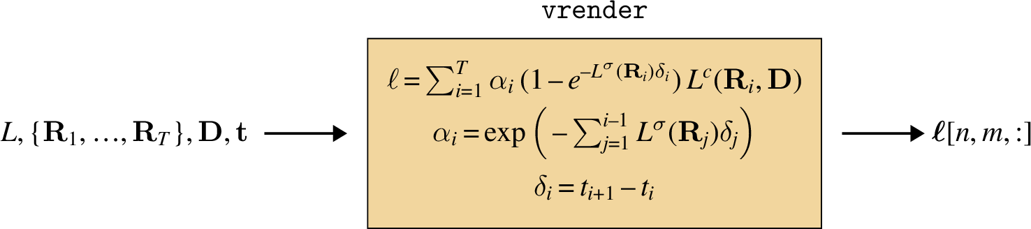
\[\begin{aligned} \ell(r) &\approx \sum_{i=1}^T \alpha_i \, (1-e^{-L^\sigma(\mathbf{R}_i)\delta_i}) \, L^c(\mathbf{R}_i, \mathbf{D})\\ &\alpha_i = \exp\Big(-\sum_{j=1}^{i-1} L^\sigma(\mathbf{R}_j)\delta_j\Big)\\ &\delta_i = t_{i+1} - t_i \end{aligned}\] where we have now replaced our continuous radiance field from Equation 45.1 with a discrete vector of samples from the radiance field, \(\{\mathbf{R}_1, \ldots, \mathbf{R}_T\}\), where \(\mathbf{R}_t = r(t)\) is the world coordinate of a point distance \(t\) along the ray \(r\).
Figure 45.7 visualizes this procedure:
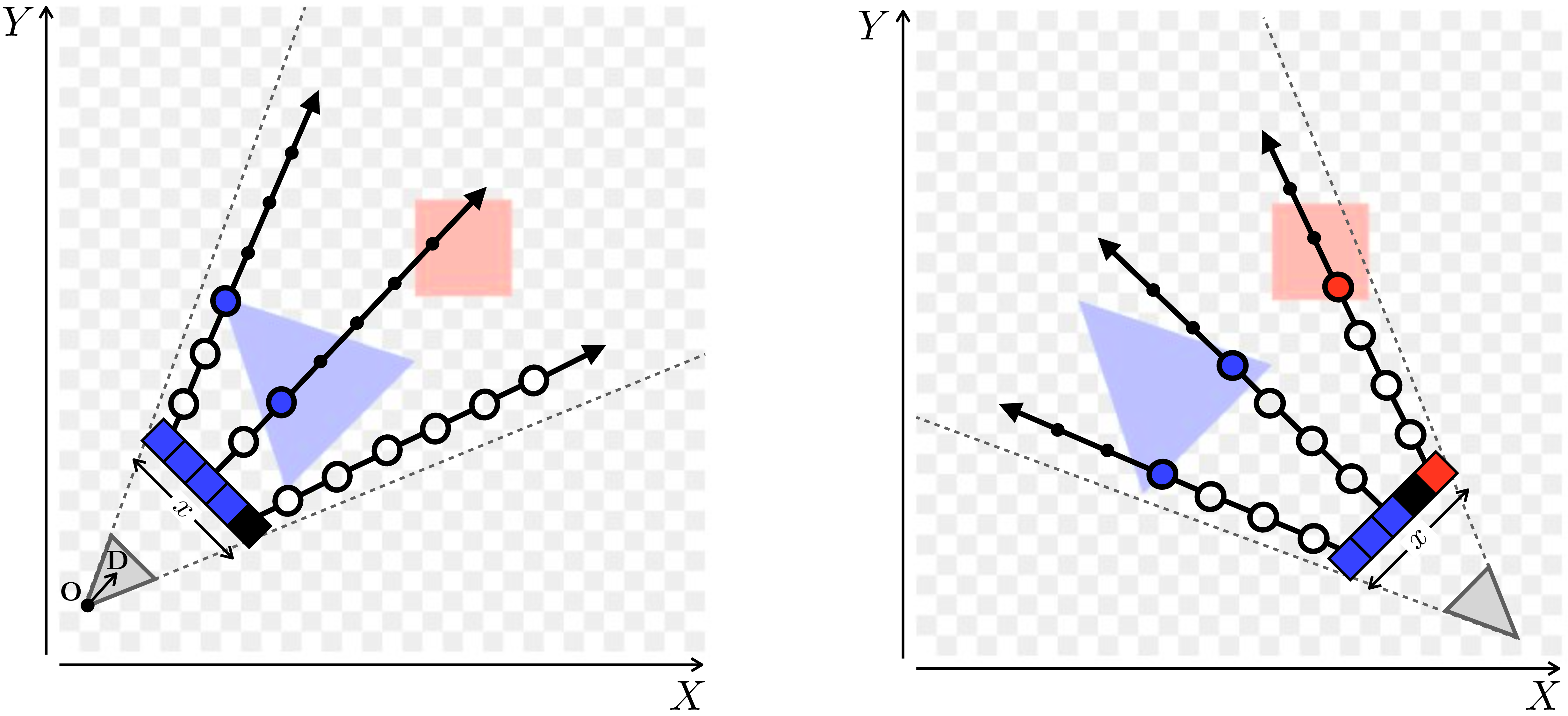
Here we have a 2D radiance field of our Flatland scene, and we are looking at it from above. We show how two cameras (gray triangles in corners) view this scene. The camera sensors are depicted as a row of five pixels, indexed by coordinate \(x\). We send a ray outward from the camera origin through each pixel to query the scene. Each ray gets sampled at the points that are drawn as circles. The size of the circle indicates the \(\alpha\) value and the color/transparency of the circle indicates the color/density of the radiance field at that point. In this scene, we have solid objects, so the density is infinite within the objects and as soon as a ray hits an object, all remaining points become occluded from view (\(\alpha\) goes to zero for the remaining points, as indicated by the circles shrinking in size).
In this figure, we took samples at evenly spaced increments along the ray. Instead, as suggested in [4], we can do better by chopping the ray into \(T\) evenly spaced intervals, then sampling one point at uniform within each of these intervals. The effect of this is that all continuous coordinates will get sampled with some probability, and therefore if we run the approximation over and over again (like we will when using it in an optimization loop; see Section 45.3.1) we will eventually take into account every point in the continuous space (they will all be supervised during fitting a radiance field to explain a scene).
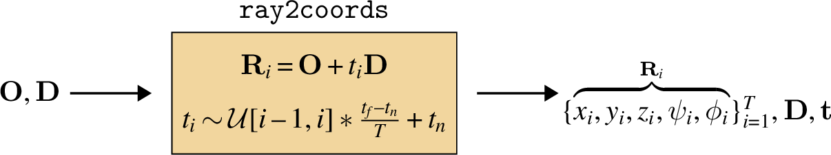
Following this strategy, for a ray whose origin is \(\mathbf{O}\) and whose direction is \(\mathbf{D}\), we compute sampled coordinates \(\{\mathbf{R}_1, \ldots, \mathbf{R}_T\}\) as follows:
\[\begin{aligned} \mathbf{R}_i &= \mathbf{O} + t_i\mathbf{D}\\ &t_i \sim \mathcal{U}[i-1,i]*\frac{t_f-t_n}{T}+t_n \end{aligned}\]
The distribution \(\mathcal{U}[a,b]\) is the uniform distribution over the interval \([a,b]\).
Now we can put all our pieces together as a series a computational modules that define the full volume rendering pipeline. Later in the chapter, we will combine these modules with other modules (including neural nets) to create a computation graph that can be optimized with backpropagation.
Our task is to compute the image \(\boldsymbol\ell\) that will be seen by a specified camera viewing the scene. We need to find the color of each pixel in this image. To find the color of a pixel, \(\boldsymbol\ell[n,m,:]\), at camera coordinate \(n,m\), the first step is to find the ray (origin \(\mathbf{O}\) and direction \(\mathbf{D}\)) that passes through this pixel. This can be done using the methods we have encountered in this book for modeling camera optics and geometry, which we will not repeat here (see Section 39.3.2. The key pieces of information we need to solve this task are the camera origin, \(\mathbf{O}_{\texttt{cam}}\), and the camera matrix, \(\mathbf{K}_{\texttt{cam}}\), that describes the mapping between pixel coordinates and world coordinates (steps for constructing \(\mathbf{K}_{\texttt{cam}}\) are given in Section 55.2.2). We apply this mapping, then compute the unit vector from the origin to the pixel to get the direction \(\mathbf{D}\) (Figure 45.8):
In this chapter, we represent RGB images as \(N \times M \times 3\) dimensional arrays.
Next we sample world coordinates along the ray, as described previously (Figure 45.9):
Finally, we use the volume rendering integral (using the quadrature rule approximation given previously) to compute the color of the pixel (Figure 45.10):
This pipeline gives a mapping from pixel coordinates to color values: \(n,m \rightarrow r,g,b\). Our task in the next section will be to explain a set of images as being the result of volume rendering of a radiance field, that is, we want to infer the radiance field from the photos.
45.5 Fitting a Radiance Field to Explain a Scene
In this section our goal is to find a radiance field that can explain a set of observed images. This is the task our denizens of Flatland have to solve as they walk around their world and try to come up with a representation of the scene they are seeing. This is the task of vision. Rendering radiance fields into images (view synthesis) is a graphics problem. We are now moving on to the vision problem, which the inverse problem and is where we really wanted to get: inferring the radiance field that renders to an observed set of images.
Concretely, our task is to take as input a set of images, along with the camera parameters for the cameras that captured those images. We will produce a parameterized radiance field as output. The full fitting procedure therefore maps \(\{\boldsymbol\ell^{(i)}, \mathbf{K}^{(i)}_{\texttt{cam}}, \mathbf{O}^{(i)}_{\texttt{cam}}\}_{i=1}^N \rightarrow L_{\theta}\).
Our objective is that if we render that radiance field, using each of the input cameras, the rendering will match the input images as closely as possible.
45.5.1 Computation Graph for Rendering an Image
Given \(L_{\theta}\), we will render an image simply using volume rendering as described previously. The entire computation graph is shown in Figure 45.11. Notice that all the modules are differentiable, which will be critical for our next step, fitting the parameters to data.

Note that the camera parameters also also need to be input into \(\texttt{pixel2ray}\) and that \(\texttt{vrender}\) also takes as input the direction \(\mathbf{D}\) and sampling points \(\mathbf{t}\) computed by \(\texttt{ray2coords}\).
45.5.2 Optimizing the Parameters of this Computation Graph
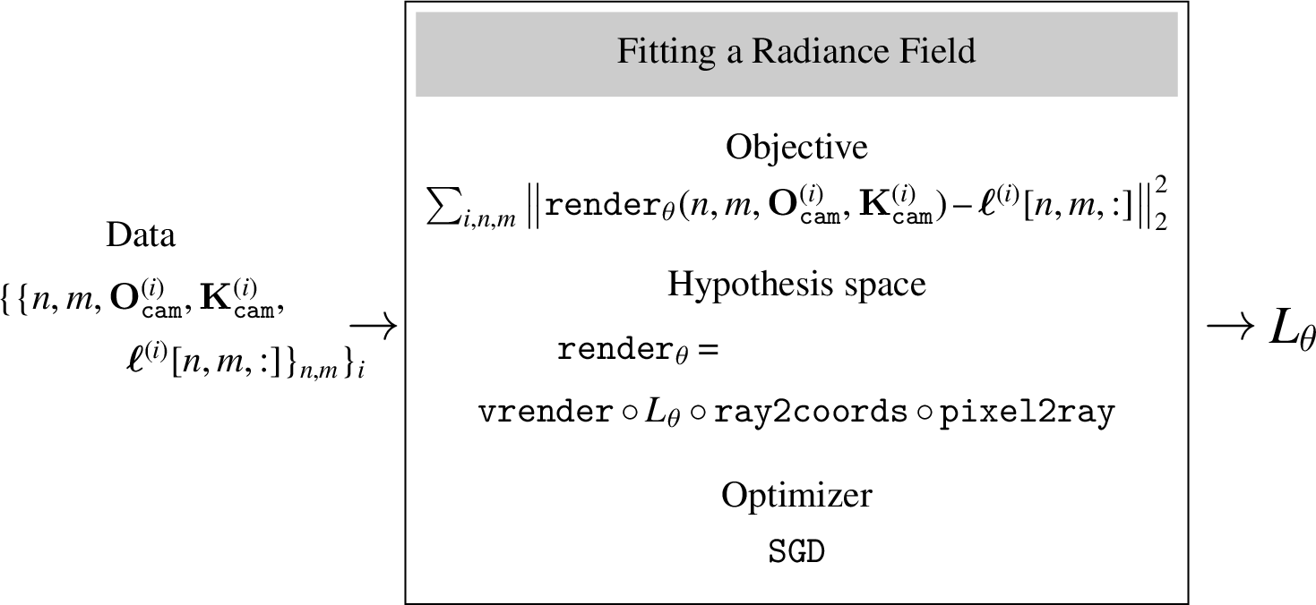
Fitting a \(L_{\theta}\) to explain the images just involves optimizing the parameters \(\theta\) to minimize the reconstruction error between the images of the radiance field rendered through \(\texttt{render}_{\theta}\) and the observed input images.
We can phrase this procedure as a learning problem and show it as the diagram below:
Fitting a radiance field to volume rendered images is very much like solving a magic square puzzle. We try to find the radiance field (the square) that integrates to the observed images (the row and column sums of the square).
From this perspective, radiance fields such as NeRF are a clever hypothesis space for constraining the mapping from inputs to outputs of a learned rendering system. Of course we could have used a much less constrained hypothesis space such as a big transformer that directly maps from input pixel coordinates to output colors, without the other modules like \(\texttt{ray2coords}\) or \(\texttt{vrender}\). However, such an unconstrained approach would be much less sample efficient and would require far more data and parameters to learn a good rendering solution (refer back to chapter Chapter 11) to recall why a more constrained hypothesis space can reduce the required amount of training data to find a good solution). However, such a solution could also be more general purpose, as it could handle optical effects that are not well captured by radiance fields.
In fact, there are two products you can get out of a fit radiance field, one for the graphics community and one for the vision community. The graphics product is a system that can render a scene from novel viewpoints. This works by just applying \(\texttt{render}_{\theta}\) (Figure 45.11) to new cameras with new viewpoints. The second product is an inferred radiance field, which tells us something about what is where in the scene. For example, the density of this radiance field can tell us the geometry of the scene, as we will see in the following example of fitting a radiance field to our Flatland scene.
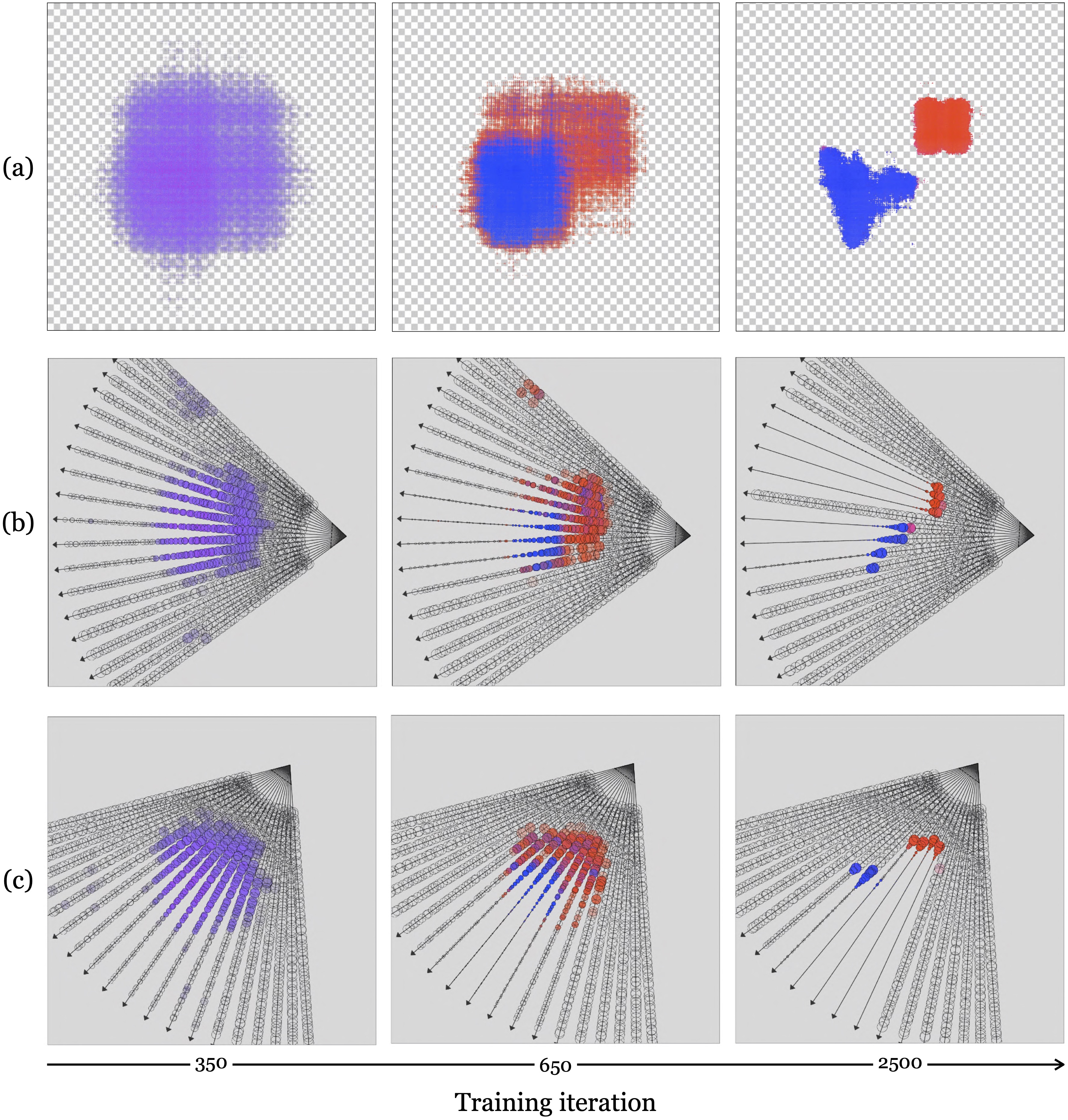
In Figure 45.12, we show several iterations of the fitting process. The top row shows the radiance field as seen from above. This is a perspective our Flatlanders cannot directly see but can infer, just like we on Earth cannot directly see the full shape of a 3D (\(X,Y,Z\)) radiance field but can infer it from images. The bottom rows show volume rendering from two different cameras. The small circles along the rays are samples of the radiance field. Their size is the \(\alpha\) value at that location along the ray, and their color and opacity are the color and density values of that location in the radiance field. Notice that initially we have a hazy cloud of stuff in the middle of the scene and over iterations it congeals into solid objects in the shapes of our Flatland denizens.
After around 2,500 steps of gradient descent, we have arrive at a fairly accurate representation of the scene. At this point, the objects’ densities are high enough that volume rendering essentially amounts to just ray casting (finding the color of the first surface we hit). So why did we use volume rendering? Not because we care about volumetric effects; in this scene there are none. Rather because it makes it possible for optimization to find the ray casting solution. With volume rendering, we have the property that small changes to the scene content yield small changes to our loss; that is, we have small but non-zero gradients. Ray casting, in contrast, is an all or none operation, and therefore small changes to scene content can yield drastic changes to the rendered images (an occluder can suddenly an the object that was previously in view of a pixel). This makes gradient-based optimization difficult with ray casting, but achievable with volume rendering. This is the second, and arguably main benefit of volume rendering that we alluded to previously (the first being the ability to model translucency and subsurface effects).
45.6 Beyond Radiance Fields: The Rendering Equation
Radiance fields are built to support volume rendering, but volume rendering has certain limitations. One major limitation of is that volume rendering does not model multi-bounce optical effects, where a photon hits a surface, bounces off, and then hits another surface, and so on. This leads to issues with how radiance fields represent shadows and reflections. Instead of a shadow being the result of a physical process where photons are blocked from illuminating one part of the scene, in radiance fields shadows get painted onto scene elements: \(L^c\) gets a darker color value in shadowed parts of the scene. If we want to change the lighting of our scene, we therefore need to update the colors in the radiance field to account for the new shadow locations, and with the radiance field representation, there is no simple way to do this (we may have to run our fitting procedure anew, this time fitting the radiance field to new images of the newly lit scene). The same is true for reflections: a radiance field will represent reflected content as painted onto a surface, rather than modeling the reflection in the physically correct way, as due to light bouncing off the surface.
Fortunately, other, more general, rendering models exist that better handle multi-bounce effects. Perhaps the most general is the rendering equation, which was introduced by Kajiya [13] in the field of computer graphics. The goal was to introduce a new formalism for image rendering by directly modeling the light scattering off the surfaces composing a scene. The rendering equation can be written as,
\[L(\mathbf{x},\mathbf{x}') = g(\mathbf{x},\mathbf{x}') \left[ e(\mathbf{x},\mathbf{x}') + \int_S \rho(\mathbf{x},\mathbf{x}',\mathbf{x}^{\prime\prime}) L(\mathbf{x}',\mathbf{x}^{\prime\prime}) d\mathbf{x}^{\prime\prime} \right] \tag{45.2}\] where \(L(\mathbf{x},\mathbf{x}')\) is the intensity of light ray that passes from point \(\mathbf{x}'\) to point \(\mathbf{x}\) (this is analogous to the plenoptic function but with a different parameterization). The function \(e(\mathbf{x},\mathbf{x}')\) is the light emitted from \(\mathbf{x}'\) to \(\mathbf{x}\), and can be used to represent light sources. The function \(\rho(\mathbf{x},\mathbf{x}',\mathbf{x}^{\prime\prime})\) is the intensity of light scattered from \(\mathbf{x}^{\prime\prime}\) to \(\mathbf{x}\) by a patch of surface at location \(x'\) (this is related to the bidirectional reflectance distribution function).
Here \(\mathbf{x}\), \(\mathbf{x}'\), and \(\mathbf{x}^{\prime\prime}\) represents a vector of world coordinates, e.g., \(\mathbf{x} = [X,Y,Z]\).
The term \(g(\mathbf{x}, \mathbf{x}')\) is a visibility function and encodes the geometry of the scene and the occlusions present. If points \(\mathbf{x}\) and \(\mathbf{x}'\) are not visible from each other, the function is 0, otherwise it is \(1/\lVert \mathbf{x}-\mathbf{x}' \rVert ^2\), modeling how energy propagates from each point.
In words of Kajiya, “The equation states that the transport intensity of light from one surface point to another is simply the sum of the emitted light and the total light intensity which is scattered toward \(\mathbf{x}\) from all other surface points.” Integrating equation (Equation 45.2) can be done using numeric methods and has been the focus of numerous studies in computer graphics.
While this rendering model is more powerful than the one radiance fields use, it is also more costly to compute. In the future, as hardware improves, we may see a movement away from radiance fields and toward models that more fully approximate the full rendering equation.
45.7 Concluding Remarks
Radiance fields try to model the light content in a scene. The ultimate goal is to model the full plenoptic function, that is, all physical properties of all the photons in the scene. Along the way to this goal, many simplified models have been proposed, and radiance fields are just one of them. Methods for modeling and rendering radiance fields build upon many of the topics we have seen earlier in this book, such as multiview geometry, signal processing, and neural networks. They appear near the end of this book because they rest upon almost all the foundations we have by now built up.