22 Filter Banks
22.1 Introduction
Although linear filters can perform a wide range of operations as we have seen in previous chapters, image understanding requires nonlinear operators. In this chapter we will study how sets of filters can be used to extract information about images. We will focus on some traditional families of filters that have been used to build image representations in the early days of computer vision and that help to understand part of the representational power of modern deep neural networks.
We will show how simple nonlinearities applied to the output of linear filters (such as the squaring nonlinearity) can be used to build useful image representations.
22.2 Gabor Filters
In Chapter 16 we discussed several useful image representations: representing an image in the frequency domain and decomposing it into amplitude and phase, and also the analysis of image content across different scales and orientations. The Fourier transform is a tool that allows us to extract that information, but only globally. For this information to be useful it needs to be localized. For instance, the analysis of orientations of local image structures can be done using image gradients (Chapter 18), which are localized in space. In fact, we made use of image derivatives in Chapter 2 to recover the three-dimensional (3D) structure of a scene. Here we will discuss another family of filters that has a long history of being used for image analysis: Gabor filters.
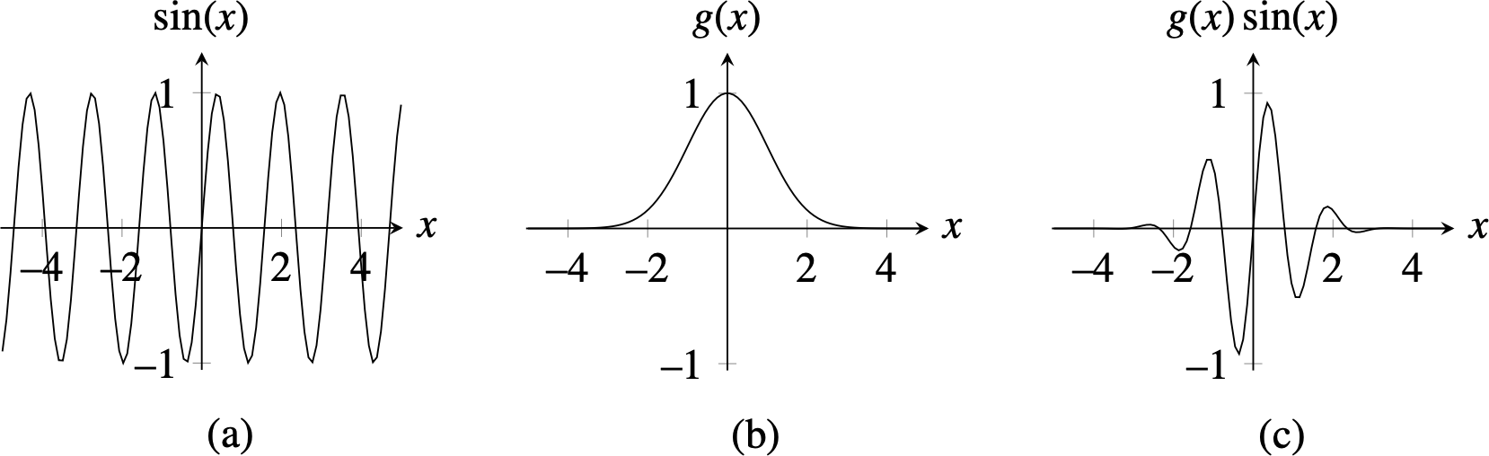
Figure 22.1 (a) shows a one-dimensional (1D) sine function. This function has infinite support. When used as a representation, the Fourier coefficients are obtained as the scalar product between the sine wave and the input image. Each Fourier coefficient involves a point-wise multiplication between the wave and the input image and then the sum of the result. As a consequence of the infinite support of the wave, one single Fourier coefficient does not tell us anything about what happens locally inside the analyzed image.
A good start for a localized image analysis is to restrict the spatial support of a sinusoidal basis function. One function that has a local support (a lot of nice properties as we discussed in Chapter 17) is the Gaussian function (Figure 22.1). The product of the Gaussian and the sine wave (or a cosine wave) gives the function with the profile shown in Figure 22.1 (c) called a Gabor filter. Gabor functions were introduced by Dennis Gabor in 1946 [1].
Gabor functions, originally proposed in 1D, were made popular as an operator for image analysis by Goesta Granlund in his paper In Search of a General Picture Processing Operator [2].
Gabor functions are localized in both the spatial and frequency domain. One remarkable property of the Gabor function is that it is the optimal function that achieves the best simultaneous localization in space and frequency.
Gabor functions can be extended to two dimensions by using 2D Gaussians and waves. We can also use complex waves (Chapter 16) as they will give us a more general form of the Gabor function.
We can multiply a complex Fourier basis function, \(\exp{ \left(j \left(u_0 x + v_0 y \right) \right)}\), by a spatially localized 2D Gaussian window, \(\exp{\left(-\frac{x^2 + y^2}{2 \sigma^2} \right) }\) to obtain a Gabor function, \(\psi(x,y)\): \[\psi(x,y;u_0,v_0) = \frac{1}{2\pi \sigma^2} \exp{\left(-\frac{x^2 + y^2}{2 \sigma^2} \right)} \exp{ \left( j \left(u_0 x + v_0 y \right) \right)} \tag{22.1}\]
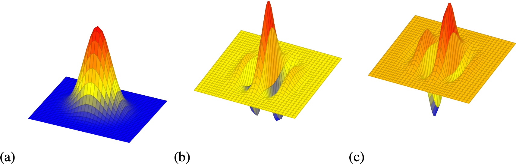
A Gabor function defined as in equation (Equation 22.1) is a complex-valued function of location and frequency. We can get the cosine and sine waves by looking at the real and imaginary components, \(\psi(x,y;u_0,v_0) = \psi_r(x,y;u_0,v_0) + j \psi_i(x,y;u_0,v_0)\) with \[\psi_r(x,y;u_0,v_0) = \frac{1}{2\pi \sigma^2} \exp{\left(-\frac{x^2 + y^2}{2 \sigma^2} \right)} \cos{ \left(u_0 x + v_0 y \right) }\] \[\psi_i(x,y;u_0,v_0) = \frac{1}{2\pi \sigma^2} \exp{\left(-\frac{x^2 + y^2}{2 \sigma^2} \right)} \sin{ \left(u_0 x + v_0 y \right) }\] Where \(\psi_r(x,y;u_0,v_0)\) and \(\psi_i(x,y;u_0,v_0)\) are the cosine and sine phase Gabor filters. Figure 22.2 shows the Gaussian window and the real and imaginary parts of the Gabor function.
The Fourier transform of a complex Gabor function is a Gaussian in the Fourier domain shifted with respect to the origin: \[\Psi(u,v; u_0,v_0) = \exp{ \left( - \left((u-u_0)^2 + (v-v_0)^2 \right) \frac{\sigma^2}{2} \right) }\]
The Gabor filter is an oriented band-pass filter.
Figure 22.3 shows the magnitude of the Fourier transform of the Gabor filters. Figure 22.3 (a) shows the cosine phase Gabor function, \(\psi_r(x,y;u_0,v_0)\), and Figure 22.3 (b) shows the sine phase Gabor function, \(\psi_i(x,y;u_0,v_0)\). Figure 22.3 (c) shows the Fourier transform of the cosine phase Gabor function, \(\Psi_r(u,v;u_0,v_0)\), and Figure 22.3 (d) shows the Fourier transform of the complex Gabor function, \(\Psi(u,v;u_0,v_0)\).
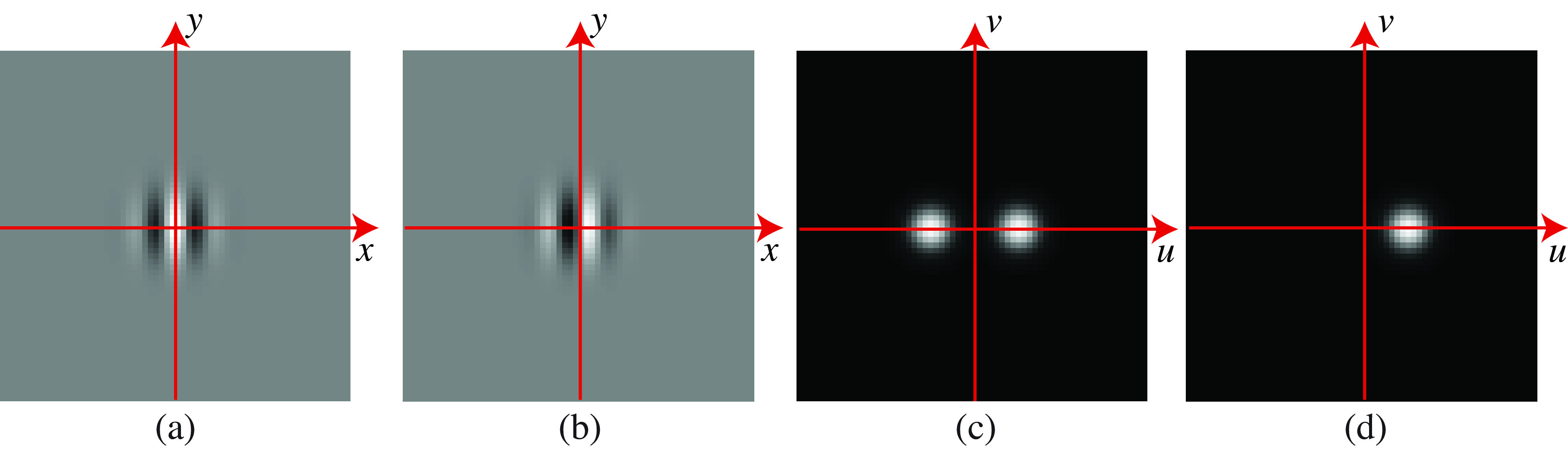
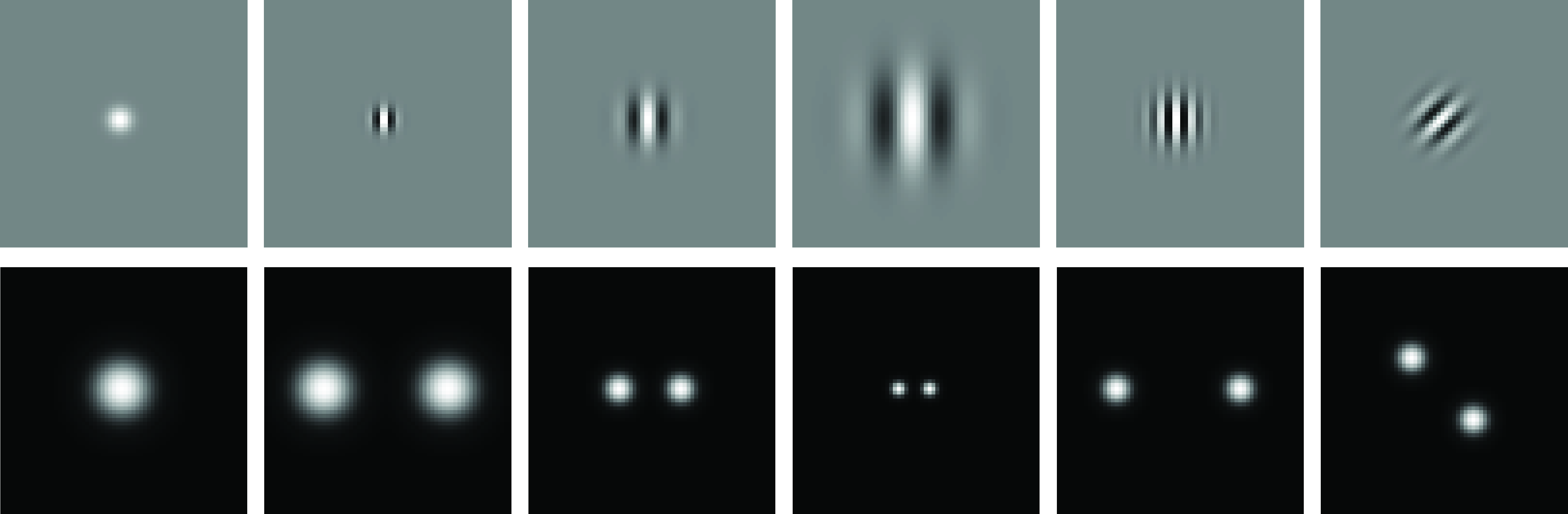
Figure 22.4 shows how the Gabor function changes when modifying its parameters (central frequency, \((u_0,v_0)\), and width, \(\sigma\)). The value of \(\sigma\) sets the locality of the window of analysis and the values of \((u_0,v_0)\) adjust the orientation of the Gabor function and frequency. A large \(\sigma\) makes the spatial extend large and the frequency extend small. A small value of \(\sigma\) has the opposite behavior. Analyzing the image with a set of Gabor functions with a large \(\sigma\) is like computing the Fourier transform of the image.
The sine phase Gabor function is zero mean. However, the cosine phase Gabor function is not zero mean. The Gaussian width \(\sigma\) has to be sufficiently large so that the Gabor function behaves like a zero mean filter. All the previous definitions are given in the continuous domain. The discrete version of the Gabor function is obtained by sampling the continuous functions.
One important characteristic of Gabor filters is that they are very similar to the shape of some cortical receptive fields found in the mammalian visual system. This provides a hint that we’re on the right track with these filters to build image representations.
Remember the description of simple and complex cells in the visual system from Chapter 1.
The convolution of the Gabor function with an image, \(\ell(x,y)\) results in an output image that depends on both space, \((x,y)\), and frequency, \((u,v)\): \[ \ell_{\psi} \left(x,y,u,v \right) = \ell\left(x,y\right) \circ \psi(x,y;u,v) \tag{22.2}\]
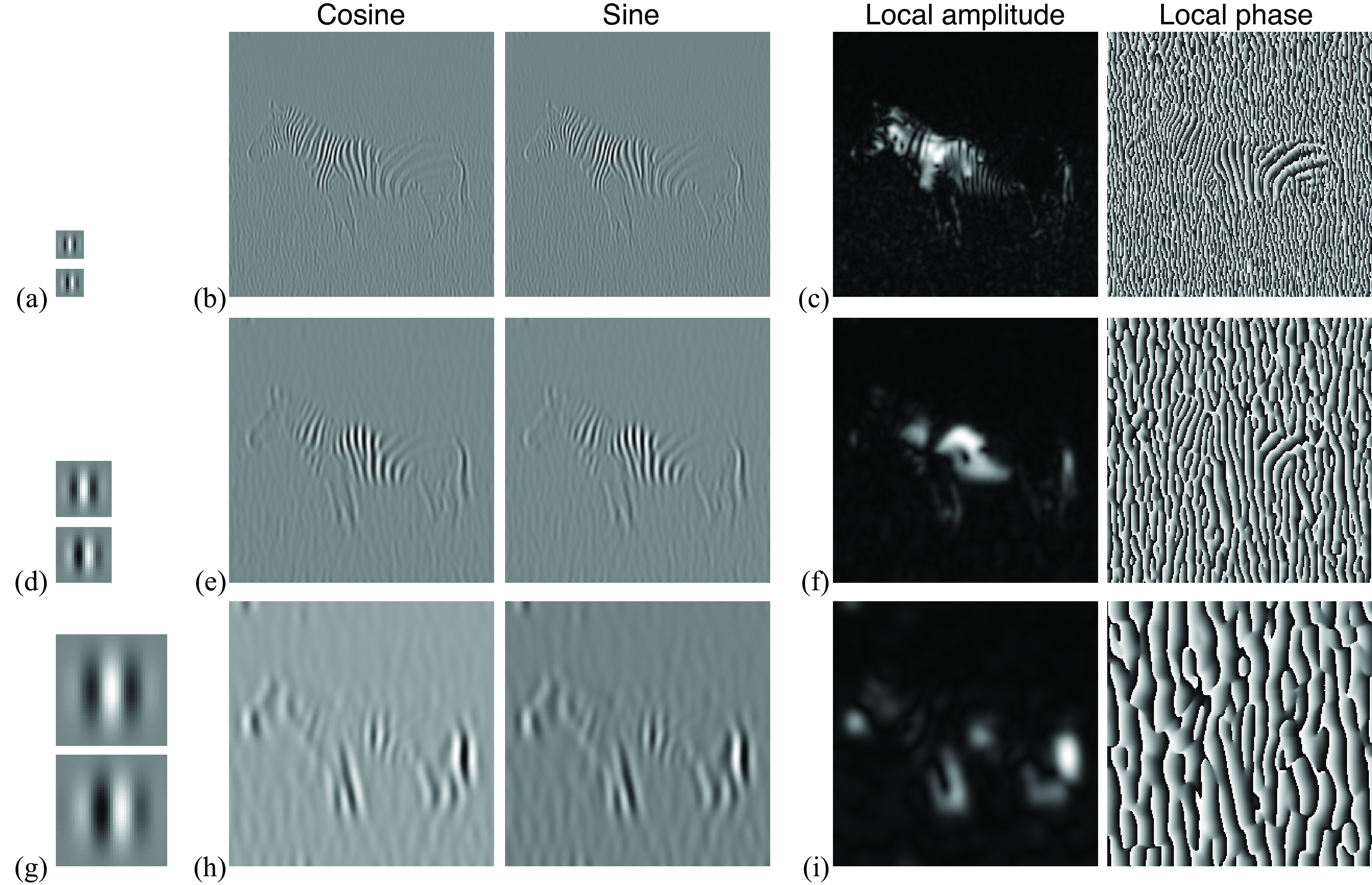
Figure 22.5 shows the result of the convolution between a picture and the cosine and sine phase Gabor functions at three different scales (\(\sigma = 2,4,8\)). In this example, the Gabor filters are tuned to detect vertical edges. Gabor filters are useful for analyzing line or edge phase structures in images. But they have many other benefits when we combine them together in quadrature pairs.
22.2.1 Quadrature Pairs and the Hilbert Transform
Pairs of filters can be in a relationship to each other that is called quadrature phase. This relationship is useful for many low-level visual processing tasks. When in quadrature phase, pairs of oriented filters can measure what is called local oriented energy, can identify contours, independently of the phase of the contour, and can measure positional changes very accurately. Let’s start with the mathematical definition of quadrature.
For notational simplicity, we’ll describe quadrature pair filters in the time domain, but they extend naturally to two or more dimensions. Consider an even symmetric zero-mean signal, \(\ell(t)\), and with Fourier transform \(\mathscr{L}(\omega)\), with \(\mathscr{L}(0)=0\) because the signal is zero-mean. In the Fourier domain, two functions, \(\mathscr{L}(\omega)\) and \(\mathscr{L}_h(\omega)\), are said to be Hilbert transform pairs if: \[\mathscr{L}_h(\omega) = \begin{cases} ~ - j \mathscr{L}(\omega) & \quad \text{if } \omega >0 \\ j \mathscr{L}(\omega) & \quad \text{if } \omega <0 \\ \end{cases}\]We now define the complex signal: \[\ell_a(t) = \ell(t) + j \ell_h(t) \tag{22.3}\]
where \(\ell_h(t)\) is the Hilbert transform of \(\ell(t)\). The signal \(\ell_a(t)\) is called the analytic signal and its Fourier transform has no negative frequency components.
It is easy to show that \[\mathscr{L}_a(\omega) = \begin{cases} ~ 2\mathscr{L}(\omega) & \quad \text{if } \omega >0 \\ 0 & \quad \text{if } \omega <0 \\ \end{cases}\]
It is interesting to write the complex signal \(\ell_a(t)\) in polar form: \[\ell_a(t) = a(t) \exp \left( j \, \theta (t) \right) \tag{22.4}\] where \(a(t)\) is the instantaneous amplitude (local amplitude) and \(\theta (t)\) is the instantaneous phase (local phase). This particular representation is common in communications theory, and it has been used to build image representations invariant to certain image structures as we will discuss in the following sections.
The extension of the Hilbert transform to images can be done in several ways. The most common approach in image processing is to define one direction, \(n\), in the frequency space and then the Hilbert transform is as follows:
\[ \mathscr{L}_h(\omega_x,\omega_y) = \begin{cases} ~ - j \mathscr{L}(\omega_x,\omega_y) & \quad \text{if } n^T \cdot (\omega_x,\omega_y) > 0 \\ j \mathscr{L}(\omega_x,\omega_y) & \quad \text{if } n^T \cdot (\omega_x,\omega_y) <0 \\ \end{cases} \]
Two band-pass filters are said to be in quadrature if the impulse responses are Hilbert transform pairs along some orientation in the frequency domain. Sine and cosine functions of the same frequency are Hilbert transform pairs, as are sine and cosine phase Gabor functions, of the same frequency and Gaussian envelope parameters. Thus, these filter pairs are also quadrature pairs. When convolving two filters in quadrature with a signal (or image) the two outputs are also in quadrature.
The quadrature in the Gabor functions is an approximation that only holds for \(\sigma\) sufficiently large. For small \(\sigma\) the filter does not form a quadrature pair. For large \(\sigma\), the real and imaginary parts of the Gabor filter (cosine and sine phase local filters) are filters in quadrature with the vector \(n=(u_0,v_0)\) pointing in the direction of the central frequency of the Gabor function.
22.2.2 Local Amplitude
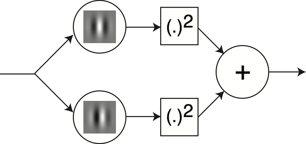
Let \(h(x,y)\) and \(q(x,y)\) be band-pass filters in quadrature, and let \(\ell_h(x,y)\) and \(\ell_q(x,y)\) be the result of convolving the signal \(\ell(x,y)\) with \(h(x,y)\) and \(q(x,y)\), respectively. Then, the squared local amplitude is a measure of the image power within the frequency bandwidth of the filters in the local neighborhood of \((x,y)\): \[a^2(x,y) = \ell_h ^2 (x,y) + \ell_q ^2 (x,y)\] Figure 22.6 shows the steps to compute the local amplitude of an input image using Gabor filters. This is like a two-layer convolutional neural network with two channels in the first layer, a squaring nonlinearity and then followed by a sum in the second layer. This very simple system can perform a number of interesting operations.
To see how useful the local amplitude is, let’s start by computing it for some simple images. If the input image is a delta, \(\ell(x,y) = \delta(x,y)\) (this is an image with a single bright dot on it), and the filters \(h\) and \(q\) are the cosine and sine phase Gabor filters, then, the local amplitude image is:
\[\begin{split} a(x,y) & = \sqrt{\ell_h ^2 (x,y) + \ell_q ^2 (x,y)} \\ & = \sqrt{\psi^2_r(x,y;u_0,v_0) + \psi^2_i(x,y;u_0,v_0)} \\ & = \frac{1}{2\pi \sigma^2} \exp{\left(-\frac{x^2 + y^2}{2 \sigma^2} \right)} \end{split} \]
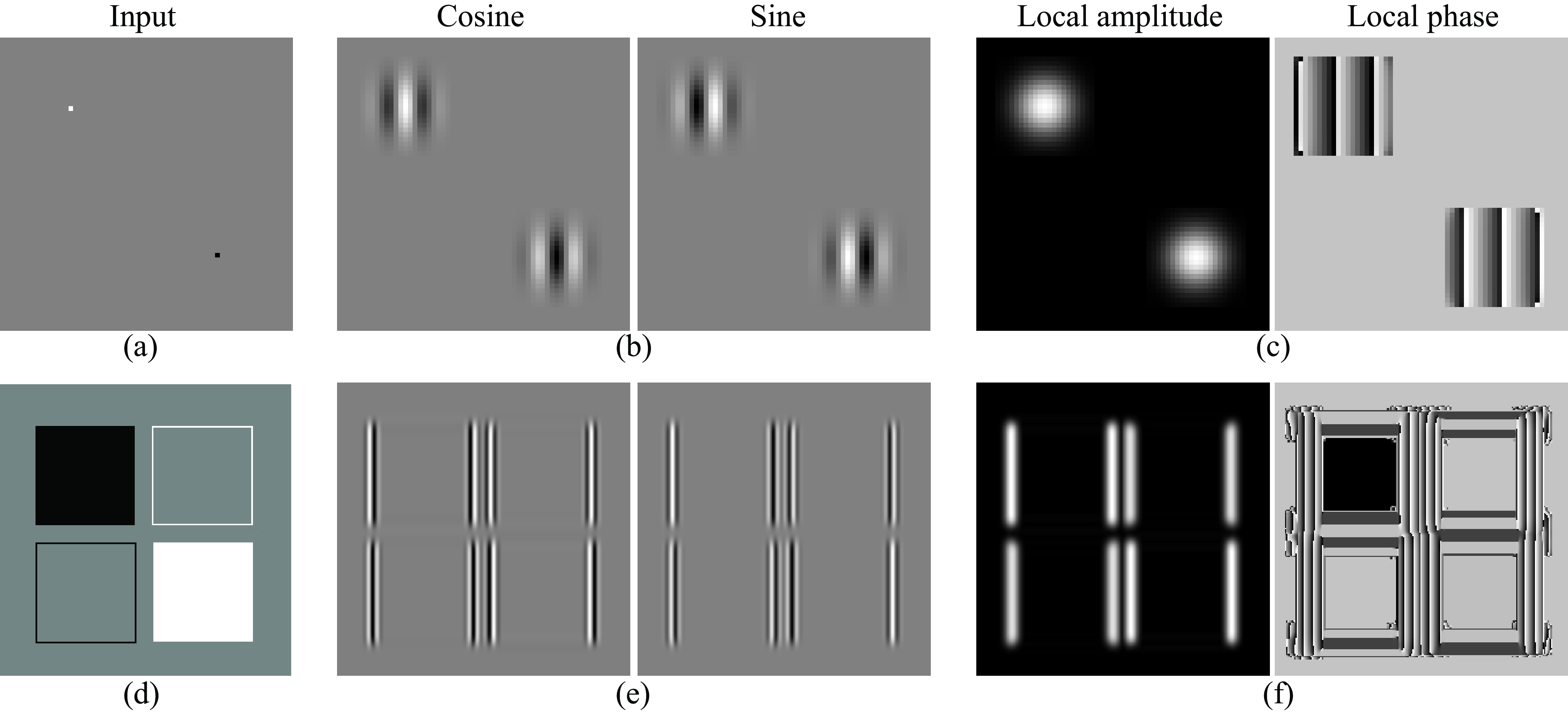
The amplitude of the delta function is the Gaussian envelope of the Gabor function. This result is independent of the contrast of the input image. For instance, if the input is \(\ell(x,y) = -\delta(x,y)\), the amplitude image does not change (it is sign invariant). Figure 22.7 (a) shows an image with two impulses of opposite signs. Figure 22.7 (b) shows the output of the cosine and sine filters, and Figure 22.7 (c) shows the local amplitude \(a(x,y)\). The local amplitude is two Gaussians centered on each impulse. Note that the sign of each impulse does not affect the sign or shape of the local amplitude. Therefore, this system is sign invariant.
The sign invariance property is especially useful when using the local amplitude to localize edges in images. Figure 22.7 (d) shows an image composed of several squares. Each square is defined by different polarities with respect to the background. Two of the squares are solid while the other two are only defined by lines. The local amplitude, Figure 22.7 (f), provides a detector for the square boundaries that is invariant to all those changes. The differences between all the squares are encoded in the local phase image as we will discuss in the following section. Figure 22.5 shows the local amplitude signal computed on real images.
One property to notice in all these examples, is that, although the images \(\ell_h(x,y)\) and \(\ell_q(x,y)\) are band-pass, the amplitude \(a (x,y)\) is a low-pass image.
22.2.3 Local Phase
The local phase is a measure of angle between the real and imaginary components (cosine and sine in the case of complex Gabor filters): \[\theta(x,y) = \angle \left[ \ell_h(x,y) + j \ell_q(x,y) \right]\] where \(\theta (x,y)\) is the instantaneous phase (local phase). This is another interesting nonlinearity although it is not commonly used in neural networks. Local image phase has been used to estimate motion [3]. This information is invariant to local changes of contrast and it is only sensitive to the local image structure.
For oriented, spatial filters, cycling through the phase of the quadrature pair of filters can generate motion along the direction of the phase change [4].
22.2.4 Gabor Filter Bank
Another useful concept is the notion of filter bank. A filter banks is a collection of filters, each tuned to extract a different image feature, and used to build an image representation.
As shown in Figure 22.3, 2D Gabor filters are selective in spatial frequency. It is very useful to work with sets of Gabor filters, each selective to a different spatial frequency so that they cover the full space of spatial frequencies.
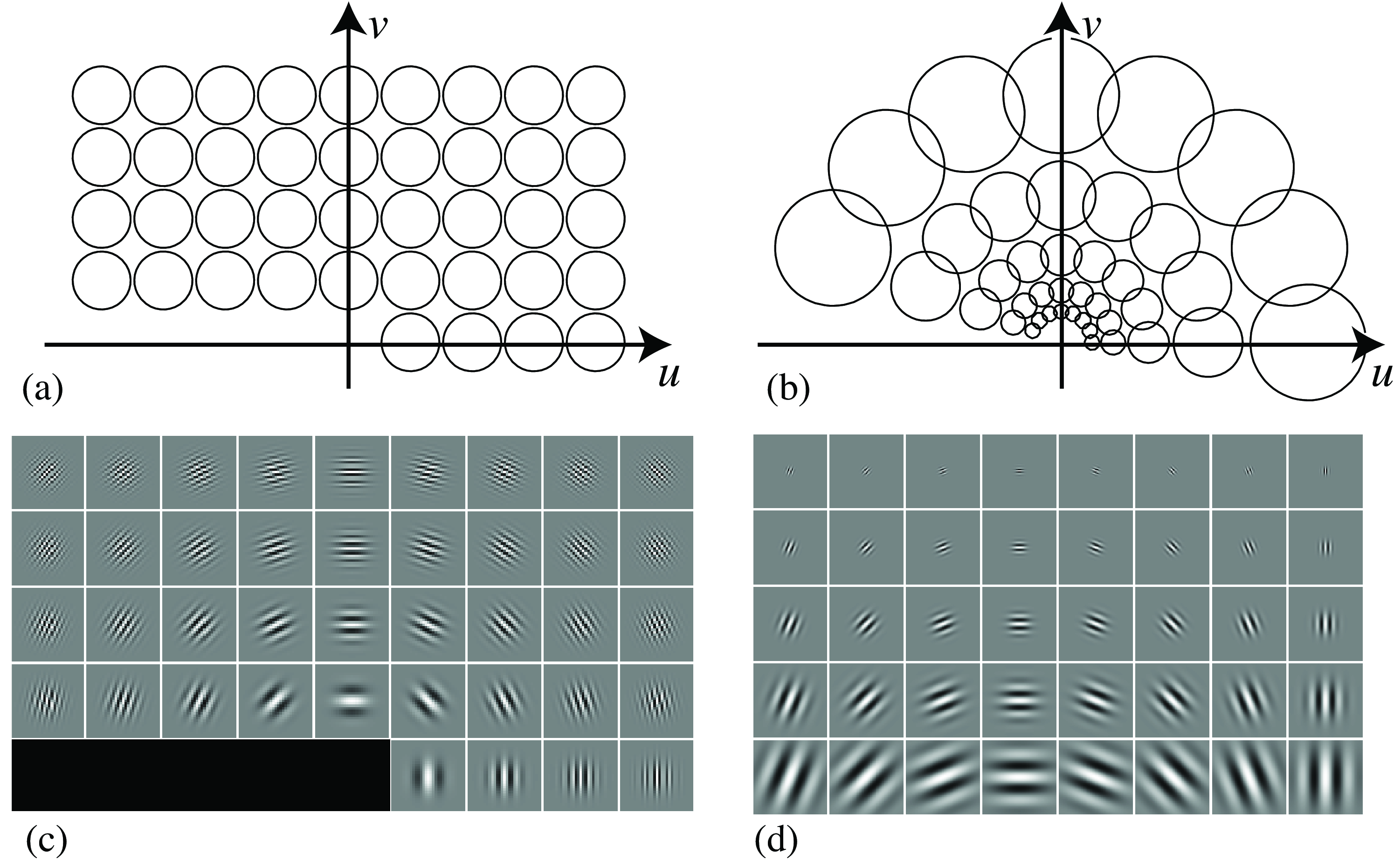
Figure 22.8 shows two different arrangements of Gabor filters. Figure 22.8 (a) shows a set of Gabor filters sampling the frequency domain using a rectangular grid. Figure 22.8 (c) shows the corresponding (cosine) Gabor kernels. All the functions have the same \(\sigma\). Figure 22.8 (b) shows a polar arrangement of Gabor functions, and Figure 22.8 (d) the spatial kernels. Here, the Gaussian width \(\sigma\) is proportional to the distance between the central frequency and the origin. This produces filters that are rotated and scaled versions of each other.
If we write in detail the convolution from equation (Equation 22.2) we can see that the convolution with a Gabor function is like doing a Fourier transform of the image after applying to it a Gaussian window: \[\begin{split} \ell_{\psi} \left(x,y,u,v \right) & = \iint \ell\left(x',y'\right) \psi(x-x',y-y';u,v) \, dx' dy' = \\ & = \iint \ell\left(x',y'\right) g(x-x',y-y') \exp \left( j \left(u (x-x') + v (y-y') \right) \right) dx' dy' = \\ \end{split}\] If we extract the term that does not depend on \((x',y')\), and we also use the symmetry of the Gaussian window, we get the following expression: \[\begin{split} & = \exp \left( j \left(u x + v y \right) \right) \iint \ell\left(x',y'\right) g(x'-x,y'-y) \exp \left(- j \left(u x' + v y' \right) \right) dx' dy' \end{split}\]
The analogous to the Fourier transform is obtained when we vary the central frequency of the Gabor function \((u,v)\). This is usually called the Gabor transform. Note that the Gabor transform is not self-inverting.
22.3 Steerable Filters and Orientation Analysis
One question that arises with oriented filters is how to change their orientation. More precisely, given a filter \(h(x,y)\), we want to transform it into a continuous function \(h(x,y, \theta)\) of angle \(\theta\). The angle \(\theta\) specifies the rotation of the original filter \(h(x,y)\).
In the case of the Gabor filters, equation (Equation 22.1), each orientation requires convolving the image with a Gabor function tuned to that orientation. But do we need to create a new Gabor function for each orientation, or can we interpolate between a fixed number of predefined oriented filter outputs? How many orientations need to be sampled?
In this section we will study a generalization of the Nyquist sampling theorem but applied to dimensions different than space.
We’d like an analog in orientation for the Nyquist sampling theorem in space: given a certain number of discrete samples in orientation (or space), can one interpolate between the samples and synthesize what would have been found from having a filter (or a spatial sample) at some arbitrary, intermediate orientation? The answer is yes, and the number of filter samples needed to interpolate depends on the form of the filter.
In Chapter 18, we described the simplest example of an oriented filter: a Gaussian derivative. As we discussed in Equation 18.4, we can synthesize a directional derivative in any direction as a linear combination of derivatives in the horizontal and vertical directions. By the linearity of convolution, that applies to the derivative applied to any filter or image, as well. It can be seen that the steering equation for the first derivative of a Gaussian filter is
\[g_{x}(x,y,\theta) = \cos(\theta) g_x(x,y) + \sin(\theta) g_y(x,y)\] where \(g_x\) and \(g_y\) are the Gaussian derivatives along \(x\) and \(y\), and \(g_{x}(x,y,\theta)\) is the derivative along the direction defined by the angle \(\theta\). The interpolation functions are \(k_1(\theta) = \cos(\theta)\) and \(k_2(\theta) = \sin(\theta)\).
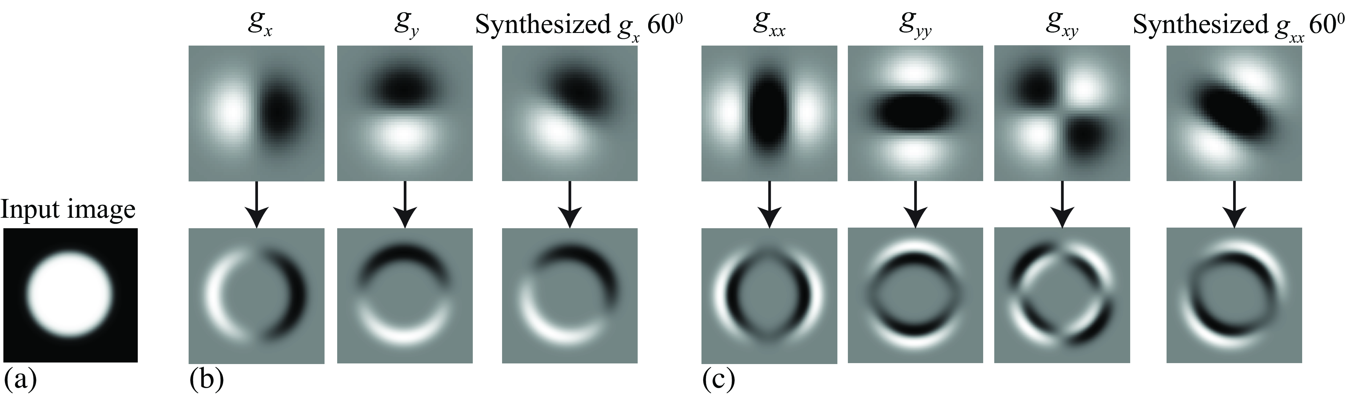
In fact, all higher order Gaussian derivatives have the same property but the number of basis filters changes. For instance, for second-order Gaussian derivatives, the steering equation is: \[\begin{split} g_{x,x}(x,y,\theta) & = g_{xx}(\cos(\theta) x - \sin (\theta) y, \sin(\theta) x + \cos (\theta)y) = \\ &= \cos^2(\theta) g_{xx}(x,y) + \sin^2(\theta) g_{yy}(x,y) - 2 \cos(\theta) \sin(\theta) g_{xy}(x,y) \end{split}\] To interpolate the derivative along any orientation requires three basis filters and the interpolation functions are \(k_1(\theta) = \cos^2(\theta)\), \(k_2(\theta) = \sin^2(\theta)\), and \(k_3(\theta) = -2\cos(\theta)\sin(\theta)\). The minus sign in \(k_3\) is due to the positive direction of \(\theta\) to be counter-clockwise. Figure 22.9 shows examples for the first- and second-order Gaussian derivatives.
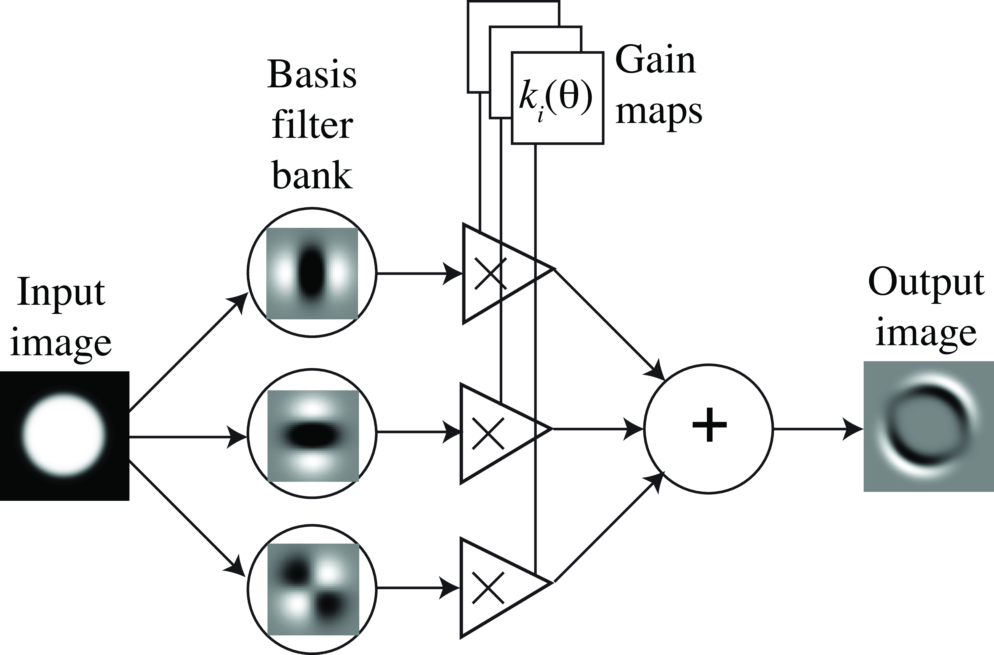
This leads to an architecture for processing images with oriented steerable filters shown in Figure 22.10. The input images pass through a set of basis filters, then the outputs of those filters are modulated with a set of gain maps (which can be different at each pixel). Those gain maps adjust the linear combinations of the basis filters to allow the input filter to be steered to the desired orientations at each position.
In the case of oriented Gabor filters it is not possible to reconstruct exactly any filter orientation by interpolating filter responses. It is interesting to study the conditions in which interpolation gives exact results.
22.3.1 Steering Theorem
Let’s make the previous observation more precise and general. How many basis filters does it take to steer any given filter? You could imagine that will depend on how sharply oriented the filter is. A circularly symmetric filter takes just one basis function to synthesize all other orientation responses, and a very narrow filter will take quite a few. This is quantified by steering theorems.
Let’s consider a filter with impulse response \(h(x,y)\). For convenience, it is better to write the filter response in polar coordinates, \(h(r,\phi)\) The steering condition is the requirement that the rotated filter, \(h(r,\phi - \theta)\), be a linear combination of a set of basis filters that are rotated versions of itself, \(h(r,\phi - \theta_m)\) with \(m \in (1,M)\). The steering condition is: \[h(r,\phi - \theta) = \sum_{m=1}^{M} k_{m}(\theta) h(r,\phi - \theta_m) . \tag{22.5}\]
If we express the filter to be steered as a Fourier series in angle (using complex exponentials for notational convenience), we have \[h(r,\phi) = \sum_{n=-N}^{N} a_n(r) \exp \left( j n \phi \right) \tag{22.6}\]
Substituting equation (Equation 22.6) into equation (Equation 22.5), we have an equation for the interpolation functions, \(k_{j}(\theta)\). The steering condition, equation (Equation 22.5), holds for functions expandable in the form of equation (Equation 22.6) if and only if the interpolation functions \(k_{j}(\theta)\) are solutions of:
\[\left[ \begin{array}{c} 1 \\ \exp (j \theta) \\ \ldots \\ \exp (j N \theta) \\ \end{array} \right] = \left[ \begin{array}{cccc} 1 & 1 & \ldots & 1 \\ \exp (j \theta_{1}) & \exp (j \theta_{2}) & \ldots & \exp (j \theta_{M}) \\ \vdots & \vdots & \vdots & \vdots \\ \exp (j N \theta_{1}) & \exp (j N \theta_{2}) & \ldots & \exp (j N \theta_{M}) \end{array} \right] \left[ \begin{array}{c} k_{1}(\theta) \\ k_{2}(\theta) \\ \vdots \\ k_{M}(\theta) \end{array} \right]. \tag{22.7}\]
Let’s check this for a simple example. Our derivative of a Gaussian filter (equation [Equation 18.1]) is \(x\) times a Gaussian. When changing to polar coordinates \(x=r \cos( \theta)\), which gives an angular distribution times a radially symmetric Gaussian when written in polar coordinates. This requires two complex exponentials to write (to create the \(\cos (\theta)\) from complex exponentials) and thus requires two basis functions to steer.
Sometimes its more convenient to think of the filters as polynomials times radially symmetric window functions (this is the case for high-order Gaussian derivatives). Then you can show that for an \(N\)-th order polynomial with even or odd symmetry \(N+1\) basis functions are sufficient [5].
Although everything has been derived in the continuous domain, steerability is a property that still holds after sampling the filter function. This is because spatial sampling and steerability are interchangeable: the weighted sum of spatially sampled function is equal to the spatial sampling of the same weighted sum of continuous basis functions.
For computational efficiency, it’s more convenient to have the basis filters all be \(x-y\) separable functions. In many cases, it’s straightforward to find such basis functions, and where it’s not, there are simple numerical methods to find the best fitting \(x-y\) separable basis set.
22.3.2 Steerable Quadrature Pairs
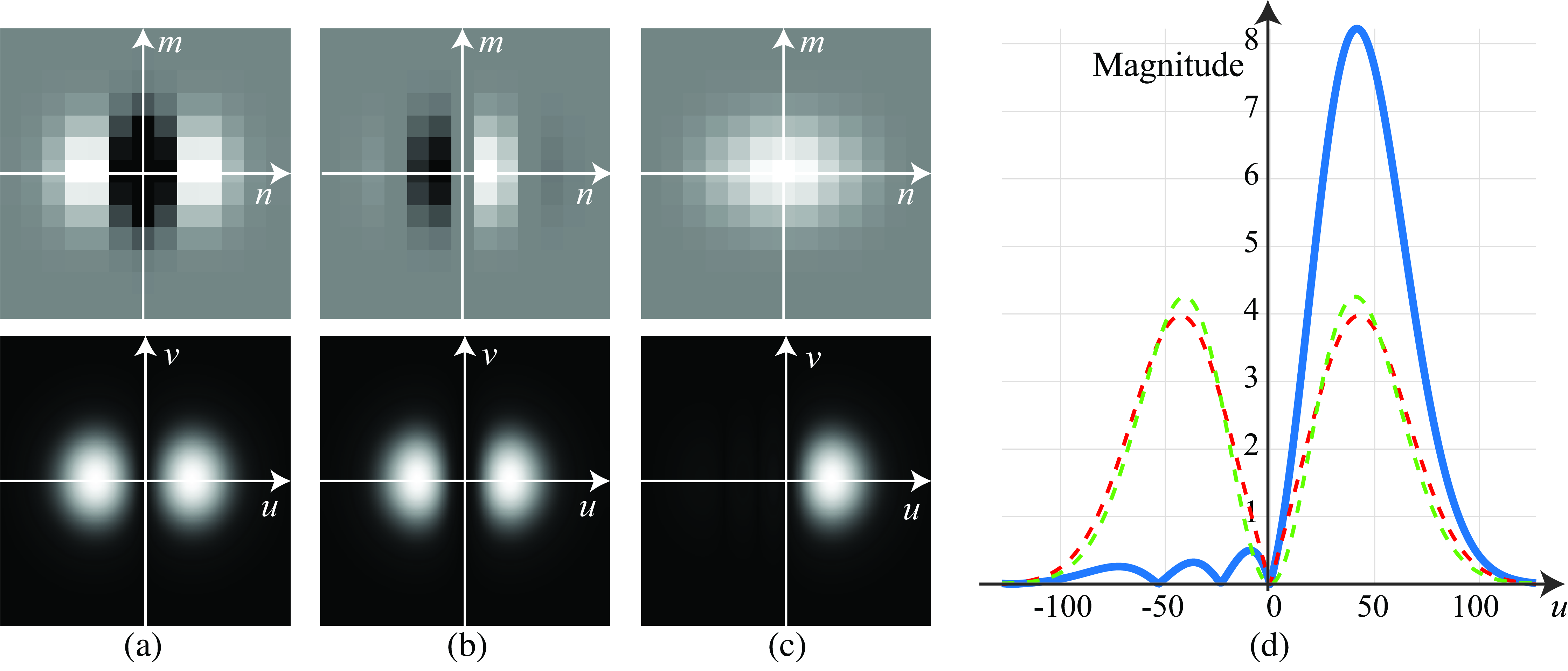
As in the case of Gabor filters, it is useful to build quadrature pairs of steerable filters. Steerable-quadrature filters allow for arbitrary shifts both in orientation and in phase. We can design such filters. For instance, let’s consider the second-order derivatives of a Gaussian with \(\sigma^2=1/2\) and normalized so that the integral over all the space of its squared magnitude equals 1: \[\begin{split} g_{xx}(x,y) &= 0.9213(2x^2-1) \exp \left(-(x^2+y^2) \right) \\ g_{xy}(x,y) &= 1.843 (x y) \exp \left(-(x^2+y^2) \right) \\ g_{yy}(x,y) &= 0.9213(2y^2-1) \exp \left(-(x^2+y^2) \right) \end{split}\] It is possible to get a good approximation to its Hilbert transform using a Gaussian times a third-order odd polynomial. The approximation to the Hilbert transform of \(g_{xx}(x,y)\) is: \[h_{xx}(x,y) = -0.9780 (-2.254 x+x^3) \exp \left(-(x^2+y^2) \right)\] where \(g_{xx}(x,y)\) and its Hilbert transform \(h_{xx}(x,y)\) have the same spectral content, but the opposite phase. Figure 22.11 analyzes the quality of the approximation. The figure shows the quadrature pair, \(g_{xx}\) and \(h_{xx}\), sampled in space and cropped into a window of \(13\times13\) pixels, and its Fourier transform. The DFT is computed by zero padding to \(256\times256\) pixels. In Figure 22.11 (a) \(g_{xx}\) is the even phase, and in Figure 22.11 (b) \(h_{xx}\) is the odd phase. Figure 22.11 (c) illustrates that the sum of their squares reveals the square of their Gaussian envelopes. Figure 22.11 (d) illustrates a section of the magnitude of their Fourier transforms along the \(u\) axis for \(v=0\). The \(h_{xx}\) is a sampled third-order polynomial approximation to the Hilbert transform of \(g_{xx}\), so their power spectra may not be exactly the same. The blue line shows the magnitude of the analytic filter \(g_{xx}+jh_{xx}\). It has double amplitude, and the content for negative frequencies is close to zero.
To steer \(h_{xx}(x,y)\) to an angle \(\theta\), this approximation requires four basis functions, and not just three as for the second-order derivative of a Gaussian. The other three functions needed are: \[\begin{split} h_2(x,y) &= -0.9780(-0.7515+x^2) y \exp \left(-(x^2+y^2) \right) \\ h_3(x,y) &= -0.9780(-0.7515+y^2) x \exp \left(-(x^2+y^2) \right) \\ h_4(x,y) &= -0.9780 (-2.254 y+y^3) \exp \left(-(x^2+y^2) \right) \end{split}\]
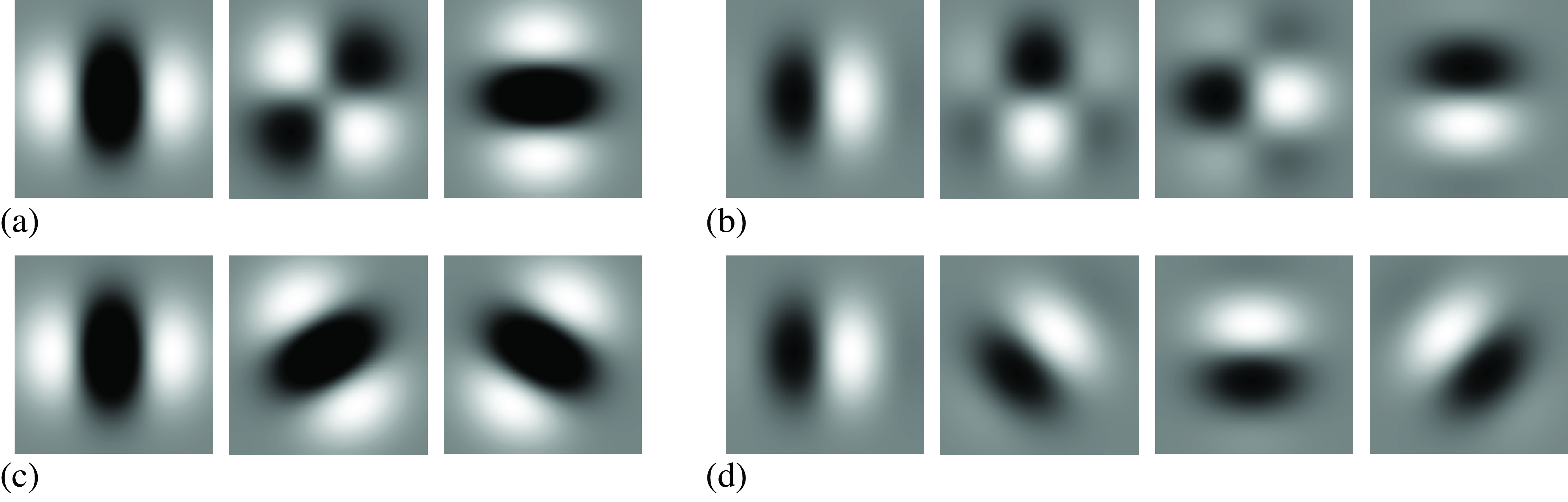
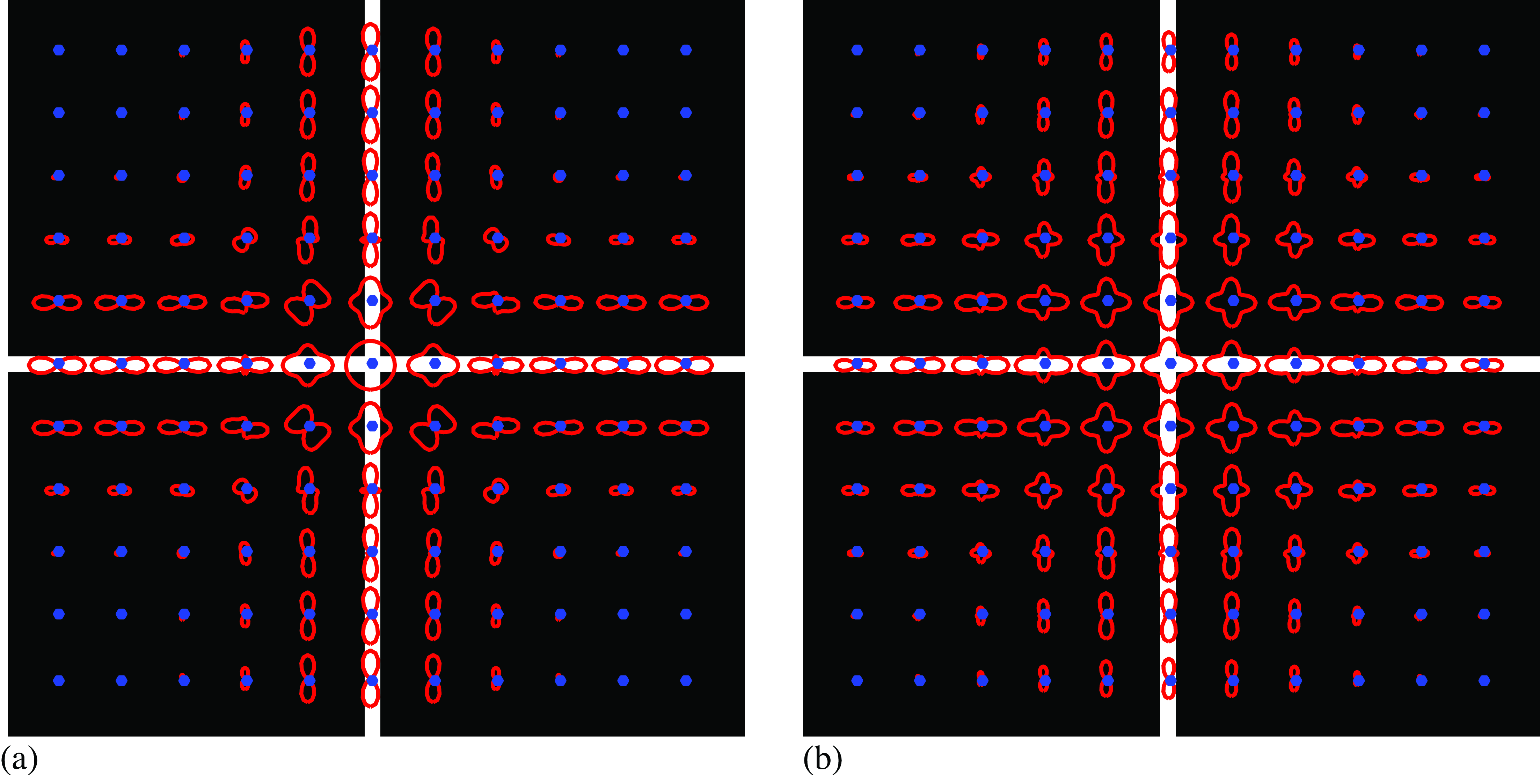
These functions have been optimized in order to be \(x-y\) separable. The basis function for steerability are not unique. For instance, figures Figure 22.12 (a and c) show two basis functions that span all rotations of \(g_{xx}\). Figure 22.12 (a) has separable filters corresponding to \(g_{xx}\), \(g_{xy}\) and \(g_{yy}\), and Figure 22.12 (c) shows three rotated versions of \(g_{xx}\) at 0, 60, and 120 degrees. Figure 22.12 (c) is a non-separable basis spanning the same space as the filters of Figure 22.12 (a). Figures Figure 22.12 (b and d) show two basis functions that span all rotations on \(h_{xx}\) spanning the same space as the filters of Figure 22.12 (b). Spatial scaling of the filters will result in changing \(\sigma\).
Putting it all together, can we compute oriented energy as a function of angle, for all angles, just from the seven basis filter responses shown in Figure 22.12. \[E(x,y,\theta) = g_{xx}(x,y,\theta)^2 + h_{xx}(x,y,\theta)^2\]
From the basis filter responses we can form polar plots of the oriented energy as a function of angle (Figure 22.13). Note some strange goings on at intersections using the \(g_{xx}\), \(h_{xx}\) filters. You might think this is a result of simply not enough angular resolution from those filters. While it’s true that the fourth-order Gaussian derivatives and their quadrature pairs don’t suffer from that problem, the \(g_{xx}\), \(h_{xx}\) filters actually do have enough angular resolution. In this case, the issue is a more subtle one.
When there are two oriented structures within the passband of the quadrature pair filters, the sum of the energies of the individual structures is not the same as the energy of the sum of the structures. Because we’re squaring to find the energies, the combination of multiple structures isn’t linear. As Figure 22.13 (a) shows, when there are two oriented structures within the passband, when the filter responses are squared, the convolution in the Fourier domain picks up extra cross-terms from the one oriented structure interacting with the other, in addition to the desired term from simply squaring all the frequency responses individually within the passband. These cross terms show up as spurious spatial frequencies in the energy term, and we can get rid of them by spatially low-pass filtering the squared oriented energy responses. Using the blurred squared basis filter responses, we get much cleaner oriented energy as a function of angle plots, even with the \(g_{xx}\), \(h_{xx}\) filters in the junctions, Figure 22.13 (b).
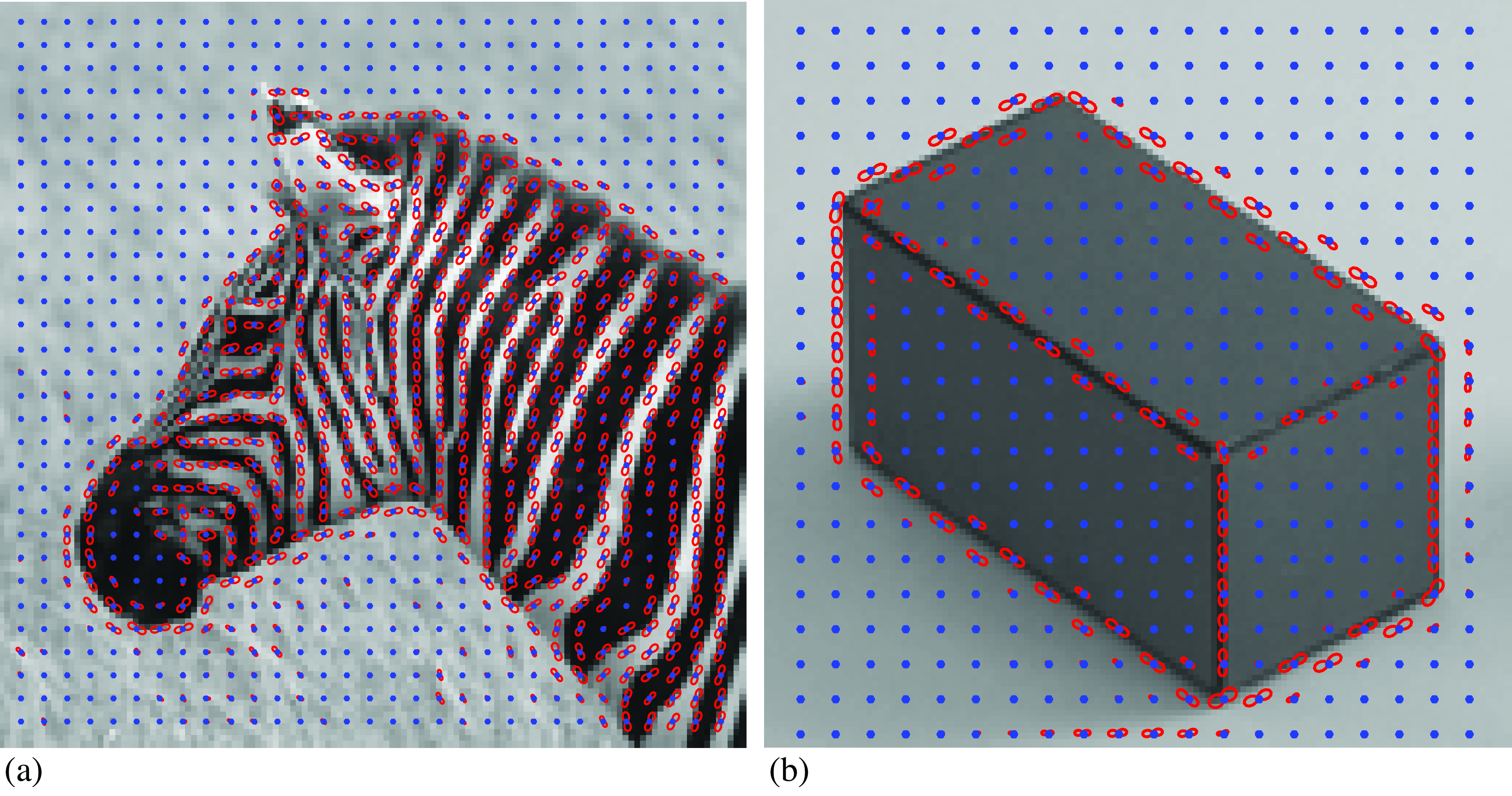
Figure 22.14 shows two examples on real images. At each pixel, the polar plots reveal the local image structure.
We can also make steerable filters in three dimensions (3D), allowing us to analyze medical volumetric data, or to process spatiotemporal volumes to measure image motion.
22.4 Motion Analysis
Spatiotemporal filter banks are a basic building block to build video understanding vision systems. In this chapter we will describe some traditional filters that are similar to filters learned when using neural networks.
22.4.1 Spatiotemporal Gabor Filters
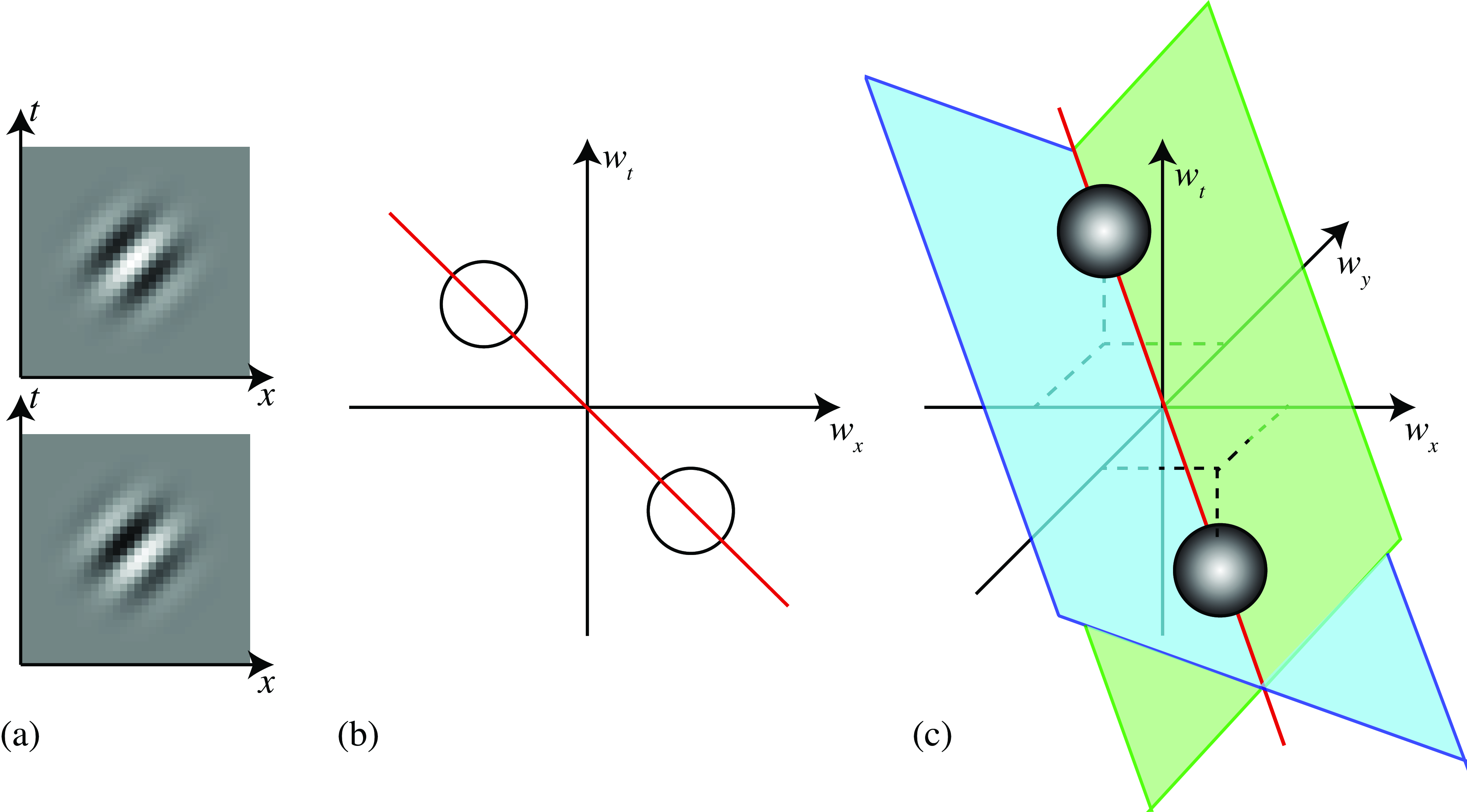
Just as we did with Gaussian derivatives, extending Gabor filter for motion analysis is a direct generalization of the \(x-y\) 2D Gabor function to a \(x-y-t\) 3D Gabor function. Figure 22.15 (a) shows a \(x-t\) (cosine and sine) Gabor function in one spatial dimension, and Figure 22.15 (b) shows a sketch of its Fourier transform. This function is selective to signals translating to the right with a speed \(v=1\), i.e. \(\ell(x-t)\). The red line in Figure 22.15 (b) shows Dirac line that contains the energy of the moving signal.
In two spatial dimensions, Figure 22.15 (c) shows the sketch of the Gabor transfer function. Note that the \(x-y-t\) Gabor filter is not selective to velocity. If we have a 2D moving signal \(\ell(x-v_xt, y-v_yt)\), the Fourier transform is contained inside a Dirac plane. Therefore, there are an infinite number of planes that will pass by the frequencies of the Gabor filter. All those planes intersect the red line shown in Figure 22.15 (c). A single Gabor filter cannot disambiguate the input velocity.
22.4.2 Velocity-Tuned Filters
How can we measure input velocity? There are many different approaches in the computer vision community for measuring motion, and we will study them in Chapter 46. Here we show that it is possible to measure motion even with the simple processing machinery that we’ve developed so far.
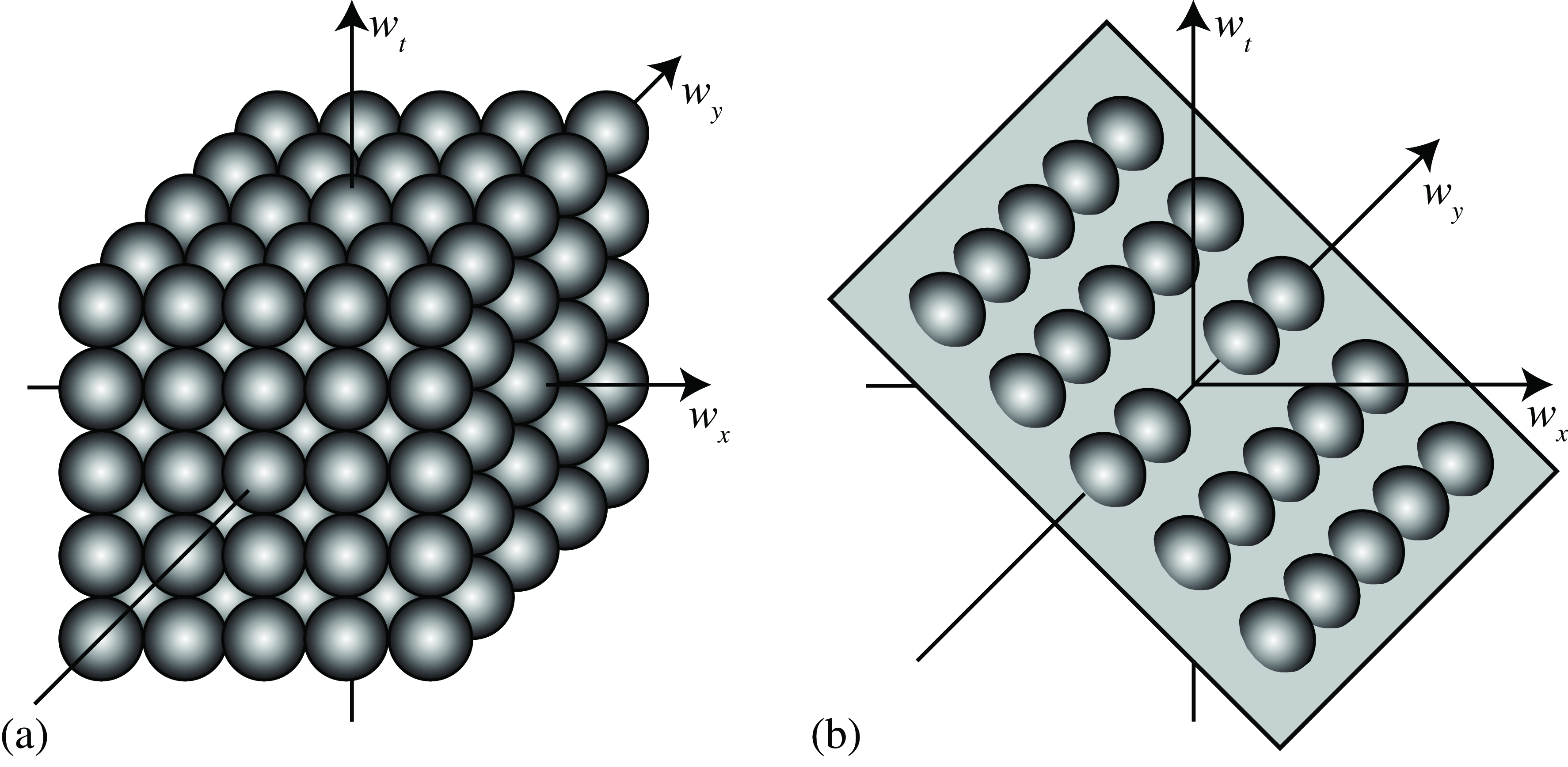
We can use quadrature pairs of oriented filters in space-time to find motion speed and direction in the video signal. We just need to find the space-time orientation of strongest response. Figure 22.16 (a) shows a set of Gabor filters sampling the space-time frequency domain. When the input contains a moving signal, we can use a set of filters to identify the plane in the Fourier domain that contains the input energy. Figure 22.16 (b) shows the subset of filters that have the strongest output for a particular input motion.
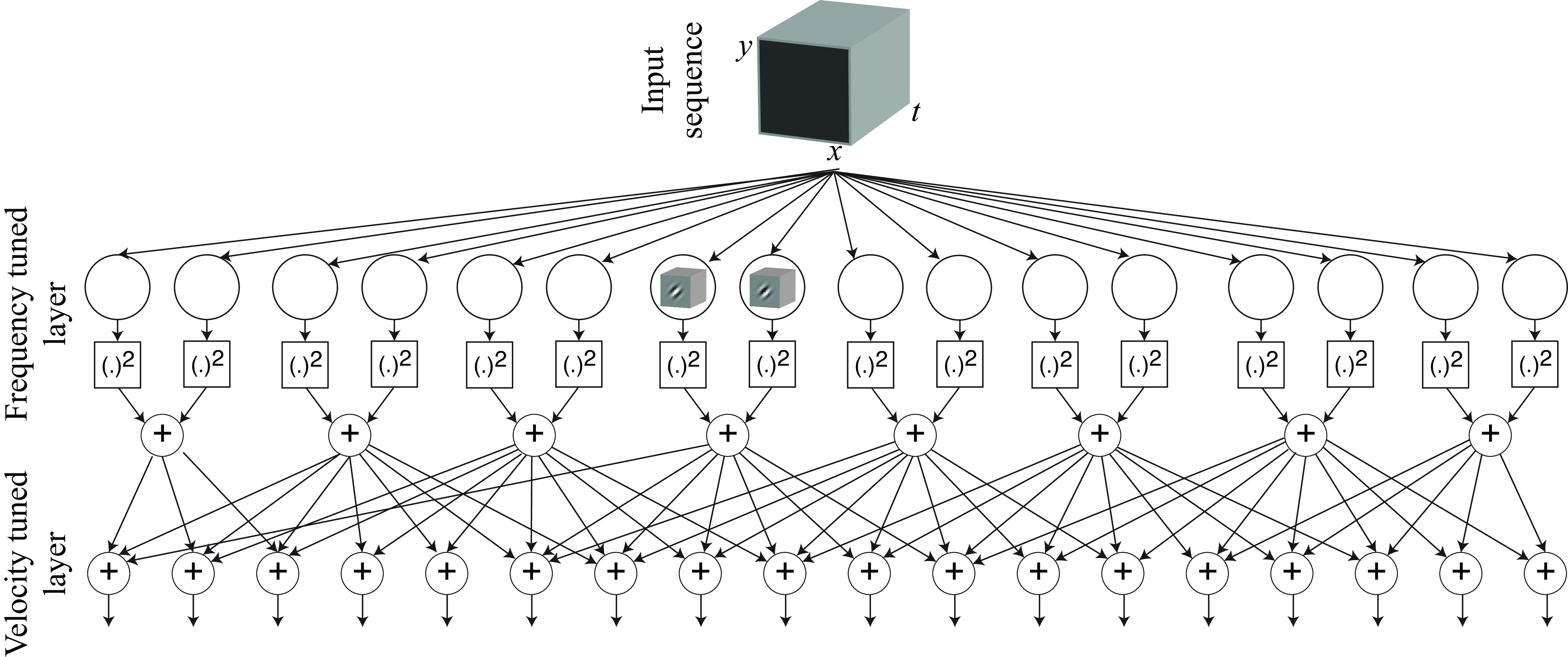
As an illustration, Figure 22.17 shows one possible architecture to create velocity-selective units. The first layer is composed by space-time Gabor filters (cosine and sine), which are frequency-selective units. Here we represent the impulse response of each filter by a small \(x-y-t\) cube. For each quadrature pair we compute the amplitude. Then amplitude outputs are combined according to form different planes in the Fourier domain to create velocity-selective outputs. A normalization layer can be added to normalize the outputs by dividing every output by the sum of all the amplitudes (not shown). The full architecture is nonlinear.
Given an input sequence, one can estimate velocity by looking at the velocity-tuned unit with the strongest response.
22.5 Concluding Remarks
In this chapter we have seen the power of using filter banks with some simple nonlinearities.
Hand-crafted filter banks started as a model of low-level vision mechanisms in humans, and became the basis to perform many visual tasks such as texture analysis [6], image segmentation [7], motion analysis [8], orientation analysis [9], image denoising [10], and many others.
These approaches had an advantage in that they were based on first principles and required no training data. However, note that performances when using hand-crafted architectures were limited. Many of the architectures we described in this chapter can be seen as precursors to many of the learning-based architectures we will discuss in subsequent chapters.
Before we dive into learning-based architectures, we will study multiscale image pyramids in the following chapter.