5 Imaging
5.1 Introduction
Light sources, like the sun or artificial lights, flood our world with light rays. These reflect off surfaces, generating a field of light rays heading in all directions through space. As the light rays reflect from the surfaces, they generally change in some attributes, such as their brightness or their color. It is those changes, after reflection from a surface, that let us interpret what we see. In this chapter, we describe how light interacts with surfaces and how those interactions are recorded with a camera.
5.2 Light Interacting with Surfaces
Visible light is electromagnetic radiation, exhibiting wave effects like diffraction. For many imaging models, however, it is helpful to introduce the abstraction of a light ray, describing the light radiation heading in a particular direction from a particular location in space (Figure 5.1). A light ray is specified by its position, direction, and intensity as a function of wavelength and polarization. In this treatment, we ignore diffraction effects.
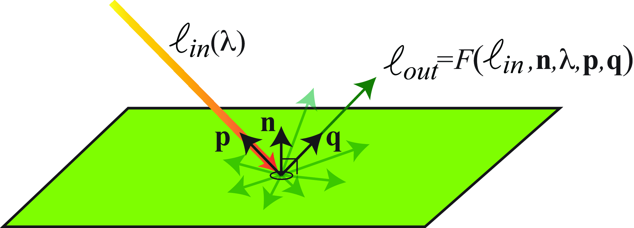
Let an incident light ray be from direction \(\mathbf{p}\) and of power, \(\ell_{\texttt{in}}(\lambda)\), as a function of spectral wavelength \(\lambda\) (). The power of the outgoing light, reflected in the direction, \(\mathbf{q}\), is determined by what is called the bidirectional reflection distribution function (BRDF), \(F\), of the surface. If the surface normal is \(\mathbf{n}\), then outgoing power is some function, \(F\), of the surface normal, the incoming and outgoing ray directions, the wavelength, and the incoming light power: \[\ell_{\texttt{out}} = F \left( \ell_{\texttt{in}}, \mathbf{n}, \lambda, \mathbf{p}, \mathbf{q} \right) \tag{5.1}\]
5.2.1 Lambertian Surfaces
In general, BRDFs can be quite complicated (see [1]), describing both diffuse and specular components of reflection. Even surfaces with completely diffuse reflections can give complicated reflectance distributions [2]. A useful approximation describing diffuse reflection is the Lambertian model, with a particularly simple BRDF, which we denote as \(F_L\). The outgoing ray intensity, \(\ell_{\texttt{out}}\), is a function only of the surface orientation relative to the incoming and outgoing ray directions, the wavelength, a scalar surface reflectance, and the incoming light power: \[ \ell_{\texttt{out}} = F_{L} \left( \ell_{\texttt{in}} (\lambda), \mathbf{n}, \mathbf{p} \right) = a \ell_{\texttt{in}}(\lambda) \left( \mathbf{n} \cdot \mathbf{p} \right), \tag{5.2}\]
where \(a\) is the surface reflectance, or albedo, \(\mathbf{n}\) is the surface normal vector, and \(\mathbf{p}\) points toward the source of the incident light. Note that the brightness of the outgoing light ray depends on the orientation of the surface relative to the incident ray, as well as the reflectance, \(a\), of the surface. For a Lambertian surface, the intensity of the reflected light is a function of the direction of the incoming light ray, but not a function of the outgoing direction of the ray, \(\mathbf{q}\).
Perfectly Lambertian surfaces are not common. The synthetic material called spectralon is the most perfectly Lambertian material.
5.2.2 Specular Surfaces
A widely used model of surfaces with a specular component of reflection is the Phong reflection model [3]. The light reflected from a surface is assumed to have three components that result in the observed reflection: (1) an ambient component, which is a constant term added to all reflections; (2) a diffuse component, which is the Lambertian reflection of Equation 5.1; and (3) a specular reflection component. For a given ray direction, \(\mathbf{q}\), from the surface, the Phong specular contribution, \(\ell_{\mbox{Phong spec}}\), is: \[\ell_{\mbox{Phong spec}} = k_s (\mathbf{r} \cdot \mathbf{q})^\alpha \ell_{\texttt{in}},\] where \(k_s\) is a constant, \(\alpha\) is a parameter governing the spread of the specular reflection, and the unit vector \(\mathbf{r}\) denotes the direction of maximum specular reflection, given by \[\mathbf{r} = 2(\mathbf{p} \cdot \mathbf{n}) \mathbf{n} - \mathbf{p}\]
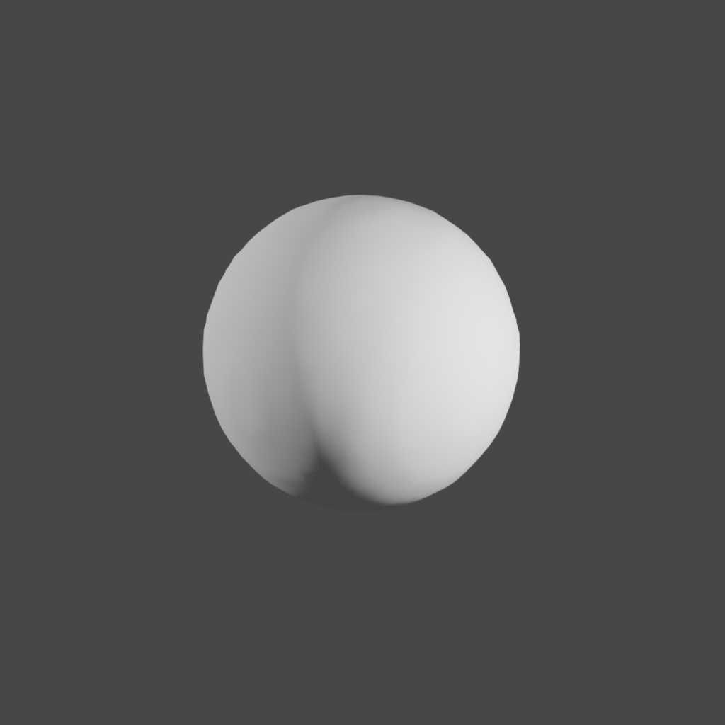
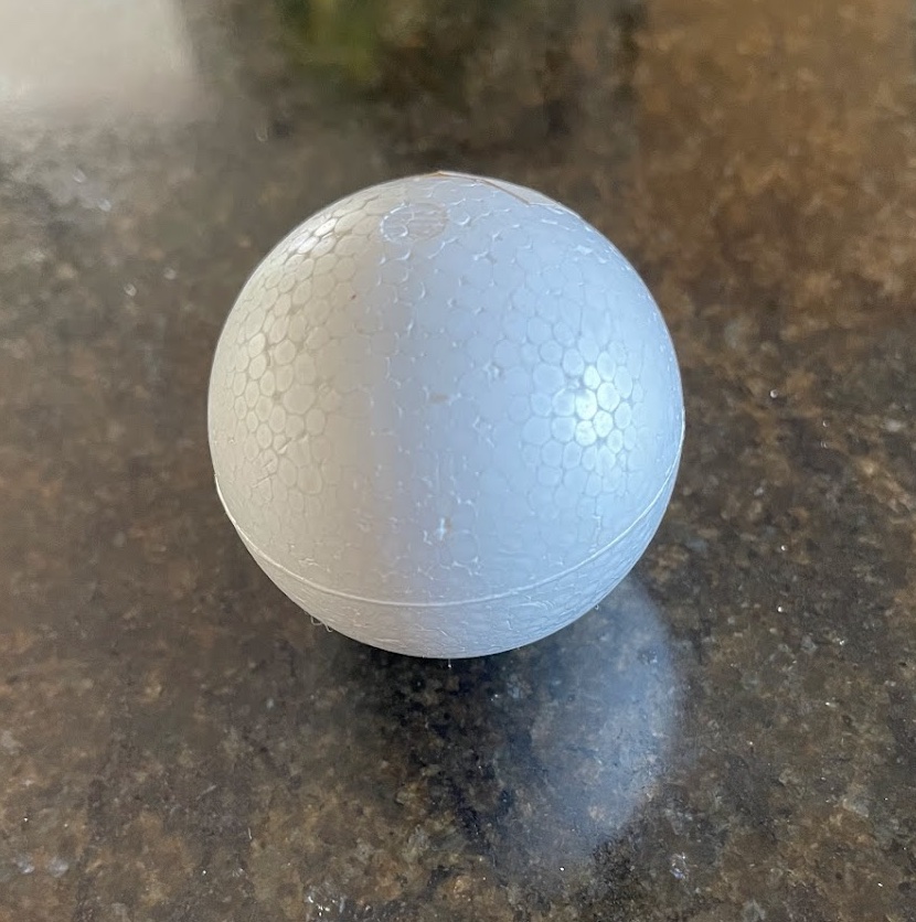
Figure 5.2 shows the ambient, Lambertian, and Phong shading components of a sphere under two-source illumination, and a comparison with a real sphere under similar real illumination.

In general, surface reflection behaves linearly: the reflection from the sum of two light sources is the sum of the reflections from the individual sources.
To associate the reflected light with surfaces in the world, we need to know which light rays came from which direction in space. That requires that we form an image, which we discuss next.
5.3 The Pinhole Camera and Image Formation
Naively, we might wonder when looking at a blank wall, why we don’t see an image of the scene facing that wall. The light reflected from the wall integrates light from every reflecting surface in the room, so the reflected intensities are an average of light intensities from many different directions and many different sources, as illustrated in Figure 5.3 (a).
Mathematically, integrating the equation for Lambertian reflections (Equation 5.1) over all possible incoming light directions \(\mathbf{p}\), we have for the intensity reflecting off a Lambertian surface, \(\ell_{\texttt{out}}\): \[\ell_{\texttt{out}} = \int_{\mathbf{p}} a \ell_{\texttt{in}}(\mathbf{p}) \cos(\mathbf{n} \cdot \mathbf{p}) \mbox{d} \mathbf{p}\] The intensity, \(\ell_{\texttt{out}}\), reflecting off a diffuse wall, thus tells us very little about the incoming light intensity \(\ell_{\texttt{in}}(\mathbf{p})\) from any given direction \(\mathbf{p}\). To learn about \(\ell_{\texttt{in}}(\mathbf{p})\), we need to form an image. Forming an image involves identifying which rays came from which directions. The role of a camera is to organize those rays, to convert the cacophony of light rays going everywhere to a set of measurements of intensities coming from different directions in space, and thus from different surfaces in the world.
Perhaps the simplest camera is a pinhole camera. A pinhole camera requires a light-tight enclosure, a small hole that lets light pass, and a projection surface where one senses or views the illumination intensity as a function of position. Figure 5.3 (b) shows the the geometry of a scene, the pinhole, and a projection surface (wall). For any given point on the projection surface, the light that falls there comes from only from one direction, along the straight line joining the surface position and the pinhole. This creates an image of what’s in the world on the projection plane.

Making pinhole cameras is easy and it is a good exercise to gain an intuition of the image projection process. The picture in Figure 5.4 shows a very simple setup similar to the diagram from Figure 5.3 (b). This setup is formed by two pieces of paper, one with a hole on it. With the right illumination conditions you can see an image projected on the white piece of paper in front of the opening. You can use this very simple setup to see the effect of changing the distance between the projection plane and the pinhole.
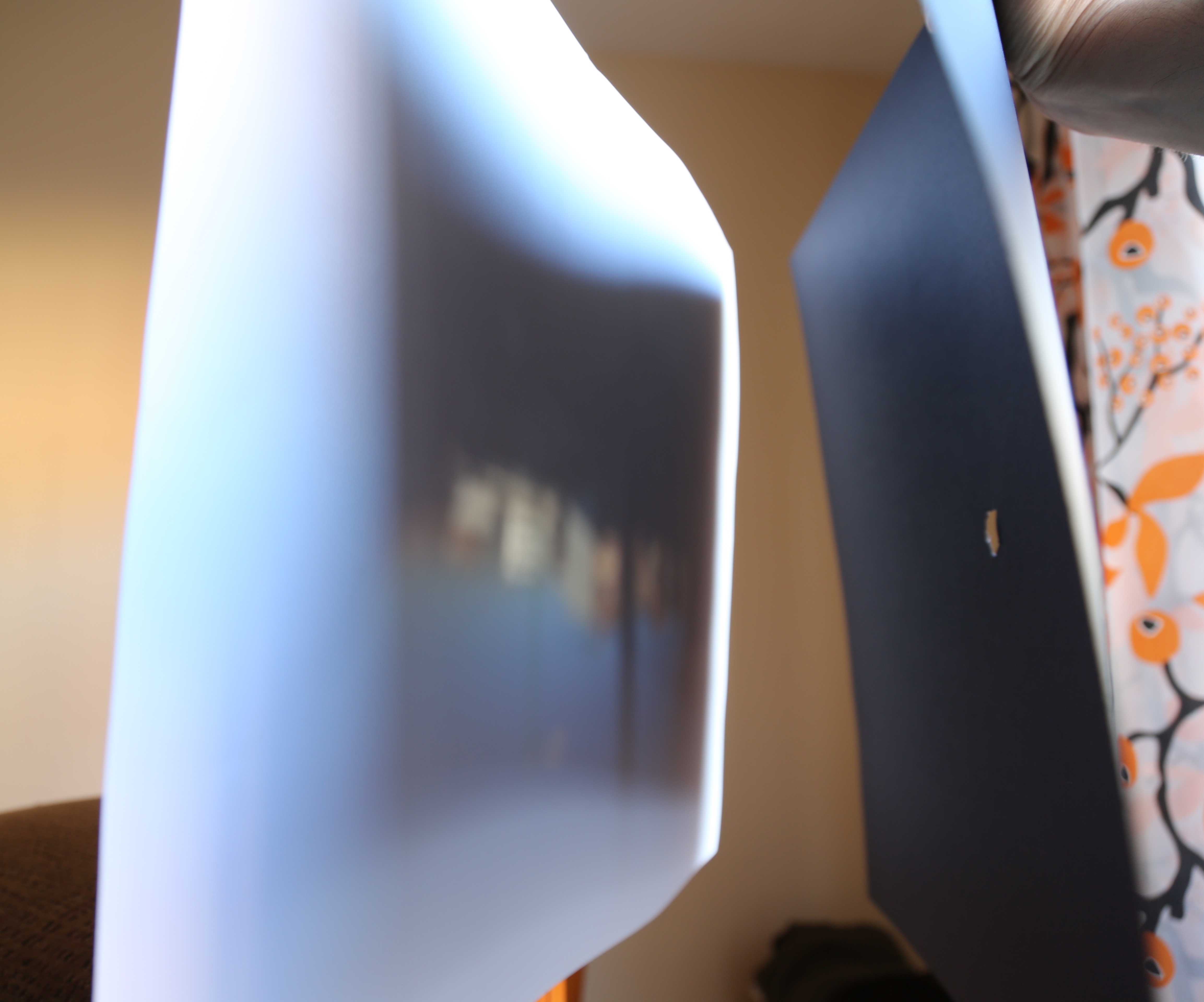
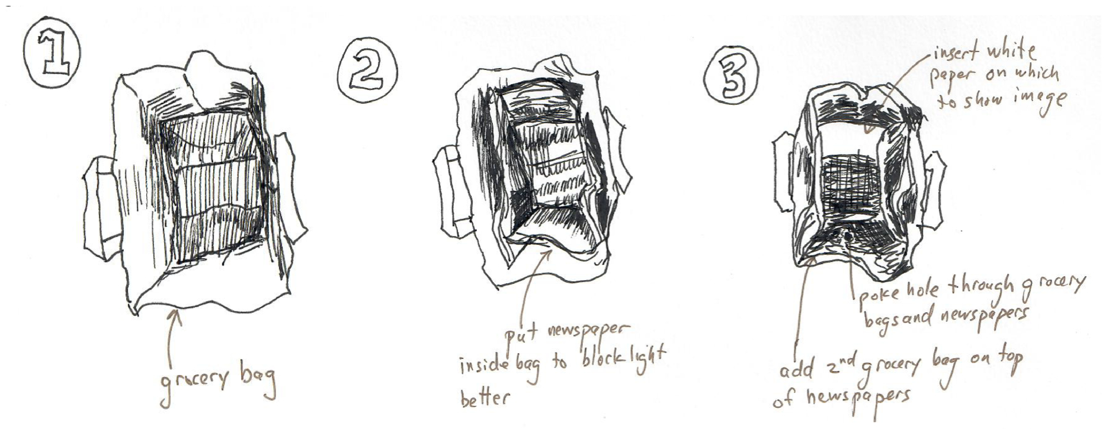
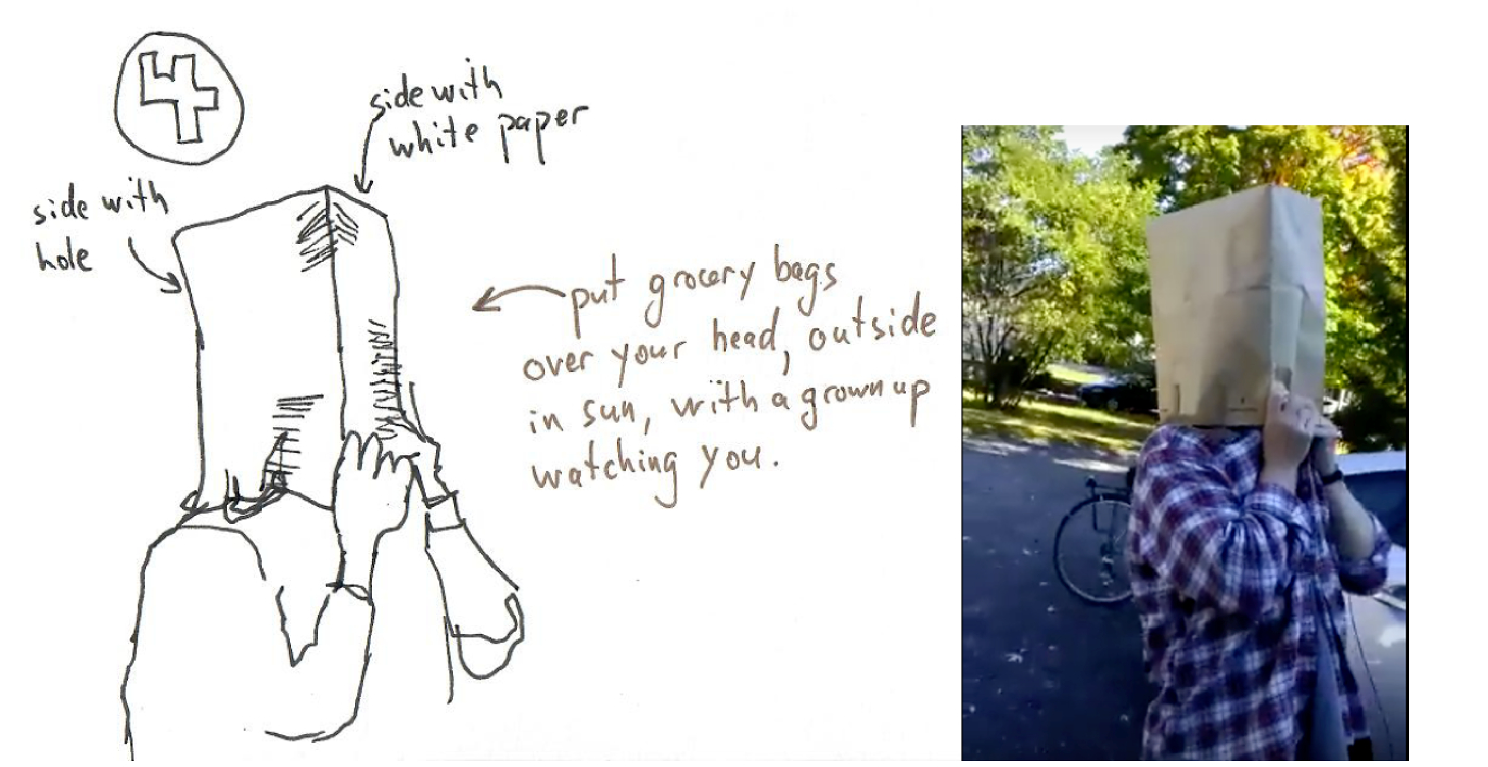
Figure 5.5 shows how to make a pinhole camera using a paper bag with a hole in it. One sticks their head inside the bag, which has been padded to be opaque. We encourage readers to make their own pinhole camera designs. The needed elements are an aperture to let light through, mechanisms to block stray light, a projection screen, and some method to view or record the image on the projection screen.
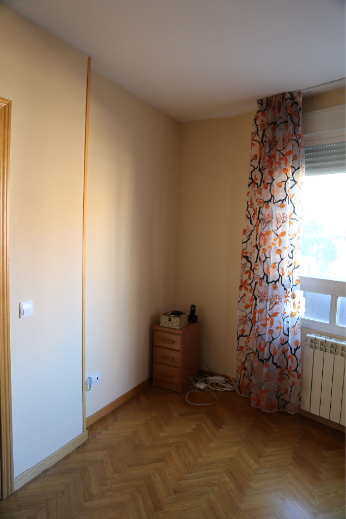
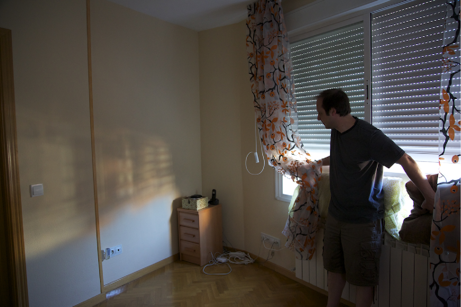
We started the section asking why there are no pictures on regular walls and explaining that, for an image to appear, we need some way of restricting the rays that hit the wall so that each location only gets rays from different directions. The pinhole camera is one way of forming a picture. But the reality is that, in most settings, light rays are restricted by accidental surfaces present in the space (other walls, ceiling, floor, obstacles, etc.). For instance, in a room, light rays are entering the room via a window, and therefore some of the rays are blocked. In general, the lower part of a wall will see the top of the world outside the window, while the top part of the wall will see the bottom part of the world outside the window. As a consequence, most walls will appear as having a faint blue tone on the bottom because they reflect the sky, as shown in Figure 5.6 (a).
The world is full of accidental cameras that create faint images often ignored by the naive observer.
5.3.1 Image Formation by Perspective Projection
A pinhole camera projects 3D coordinates in the world to 2D positions on the projection plane of the camera through the straight line path of each light ray through the pinhole (Figure 5.3). The simple geometry of the camera lets us identify the projection by inspection. The sketch in Figure 5.7 shows a pinhole camera and the relevant terminology.
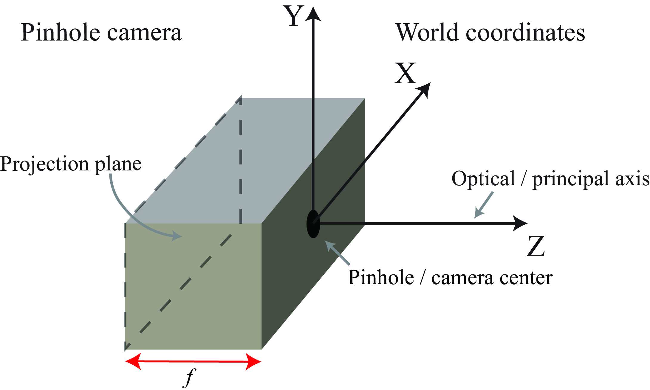
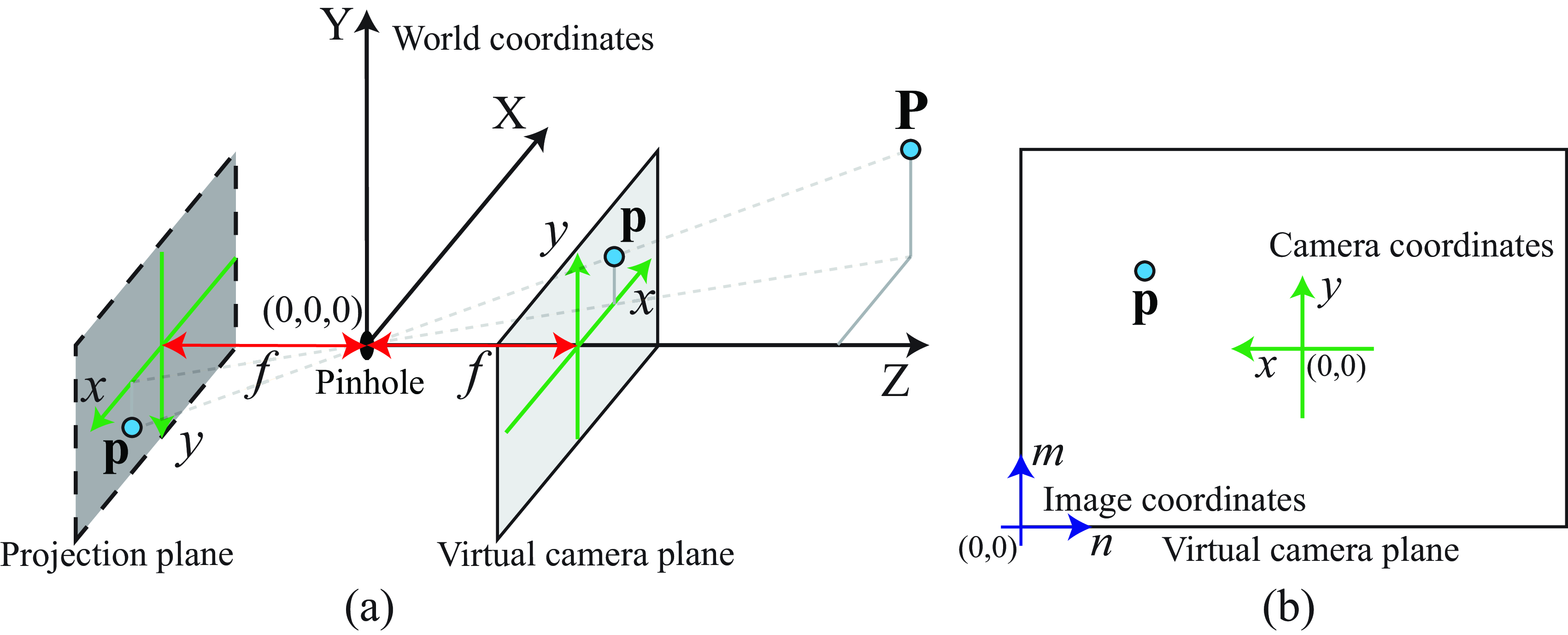
Figure 5.8 shows the pinhole camera of Figure 5.7 but with the box removed, leaving visible the projection plane. Figure 5.8 shows the definition of the three coordinate systems that we will use:
World coordinates. Let the origin of a World Cartesian coordinate system be the camera’s pinhole. The coordinates of 3D position of a point, \(\mathbf{P}\), in the world will be \(\mathbf{P} = (X, Y, Z)\), where the Z axis is perpendicular to the camera’s sensing plane (projection plane).
Camera coordinates in the virtual camera plane. The camera projection plane is behind the pinhole and at a distance \(f\) of the origin. Let the coordinates in the camera projection plane, \(x\) and \(y\), be parallel to the world coordinate axes \(X\) and \(Y\) but in opposite directions, respectively. For simplicity, it is useful to create a virtual camera plane that is radially symmetrical to the projection plane with respect to the origin and it is placed in front of the camera ([a]). This virtual camera plane will create a projected image without the inversion of the image. The coordinates in the virtual camera plane will have the same sign as the world coordinates, that is, with the same \(x\),\(y\) coordinates (i.e., both images are identical apart from a flip).
Image coordinates, shown in , are typically measured in pixels. Both the camera coordinate system \((x,y)\) and the image coordinate system \((n,m)\) are related by an affine transform as we will discuss later.
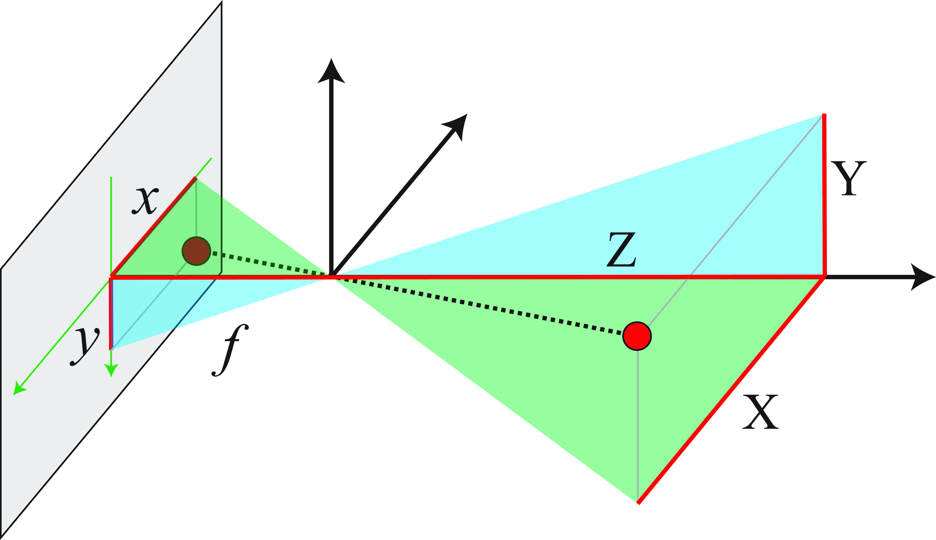
If the distance from the sensing plane to the pinhole is \(f\) (see Figure 5.9) then similar triangles gives us the following relations:
\[\begin{align} x &= f \frac{X}{Z} \end{align} \tag{5.3}\]
\[\begin{align} y &= f \frac{Y}{Z} \end{align} \tag{5.4}\]
Thales of Miletus, 624 B.C., introduced the notion of similar triangles. It seems he used this to measure the height of Egypt pyramids, and the distance to boats in the sea.
Equations Equation 5.3 and Equation 5.4 are called the perspective projection equations. Under perspective projection, distant objects become smaller, through the inverse scaling by \(Z\). As we will see, the perspective projection equations apply not just to pinhole cameras but to most lens-based cameras, and human vision as well.
Due to the choice of coordinate systems, the coordinates in the virtual camera plane have the \(x\) coordinate in the opposite direction than the way we usually do for image coordinates \((m,n)\), where \(m\) indexes the pixel column and \(n\) the pixel row in an image. This is shown in Figure 5.8 (b). The relationship between camera coordinates and image coordinates is \[\begin{aligned} n &= - a x + n_0\\ m &= a y + m_0 \label{eq-cameratoimagecoordinates} \end{aligned}\] where \(a\) is a constant, and \((n_0, m_0)\) is the image coordinates of the camera optical axis. Note that this is different than what we introduced a simple projection model in in the framework of the simple vision system in Chapter 2. In that example, we placed the world coordinate system in front of the camera, and the origin was not the location of the pinhole camera.
Biological systems rarely have eyes that are built as pinhole cameras. One exception is the Nautilus, which has evolved a pinhole eye (without any lens).
5.3.2 Image Formation by Orthographic Projection
Perspective projection is not the only feasible projection from 3D coordinates of a scene down to the 2D coordinates of the sensor plane. Different camera geometries can lead to other projections. One alternative to perspective projection is orthographic projection. Figure 5.10 shows the geometric interpretation of orthographic (or parallel) projection.
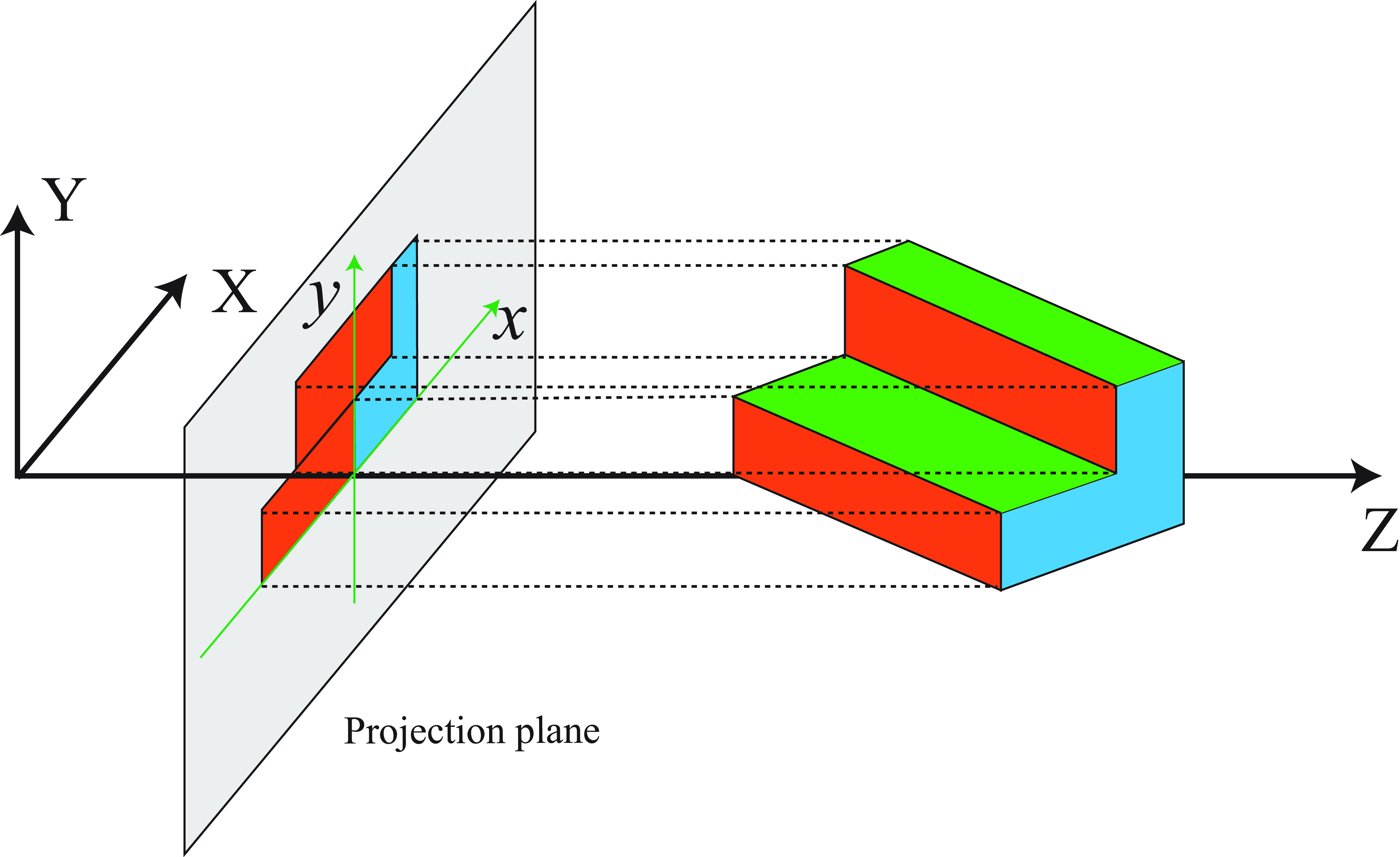
In this projection, as the rays are orthogonal to the projection plane, the size of objects is independent of the distance to the camera. The projection equations are generally written as follows: \[\begin{aligned} x &= k X \nonumber \\ y &= k Y \end{aligned} \tag{5.5}\] where the constant scaling factor \(k\) accounts for change of units and is a fixed global image scaling.
Orthographic projection is a good model for telephoto lenses, where the apparent size of objects in the image is roughly independent of their distance to the camera. We used this projection when building the simple visual system in Chapter 2.
Orthographic Projection is a correct model when looking at an infinitely far away object that is infinitely zoomed in, as discussed in Chapter 2.
The next section provides another example of a camera producing an orthographic projection.
5.3.3 How to Build an Orthographic Camera?
Can we build a camera that has an orthographic projection? What we need is some way of restricting the light rays so that only perpendicular rays to the plane illuminate the projection plane.
One such camera is the soda straw camera, shown in Figure 5.11, which you can easily build. The example shown in (c) used around 500 straws.
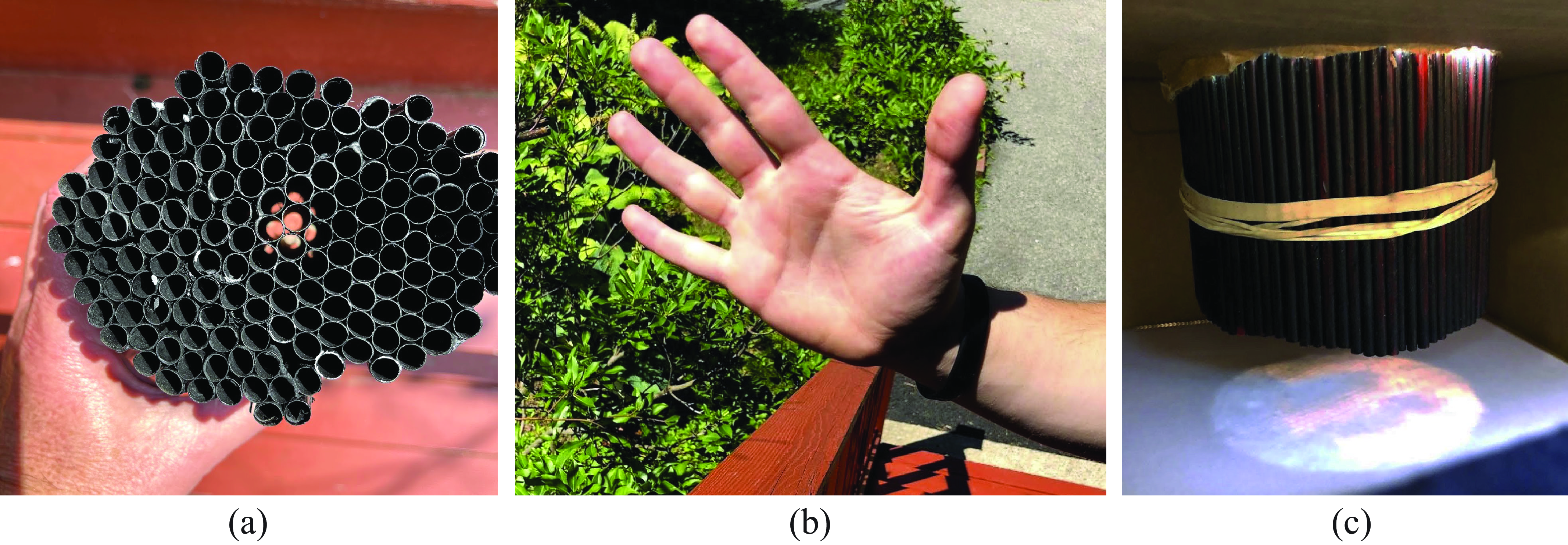
A set of parallel straws allow parallel light rays to pass from the scene to the projection plane, but extinguish rays passing from all other directions. It works better if the straws are painted black to reduce internal reflections that might capture light rays not parallel to the straws, resulting in a less sharp picture.
Figure 5.11 (c) shows the resulting image when imagining the scene shown in Figure 5.11 (b). The straw camera doesn’t invert the image as the pinhole camera does and objects do not get smaller as they move away from the camera. The image projection is orthographic, with a unity scale factor; the object sizes on the projection plane are the same as those of the objects in the world.
A larger straw camera has been built by Michael Farrell and Cliff Haynes [4] with an impressive 32,000 drinking straws.
Another implementation of an orthographic camera is the telecentric lens that combines a pinhole with a lens.
5.4 Concluding Remarks
Light reflects off surfaces and scatters in many directions. Pinhole cameras allow only selected rays to pass to a sensing plane, resulting in a perspective projection of the 3D scene onto the sensor. Other camera configurations can give other image projections, such as orthographic projections.
At this point, it is a good exercise to build your own pinhole camera and experiment with it. Building a pinhole camera helps in acquiring a better intuition about the image formation process.