7 Cameras as Linear Systems
7.1 Introduction
Lens-based and pinhole cameras are special-case devices where the light falling on the sensors or the photographic film forms an image. For other imaging systems, such as medical or astronomical systems, the intensities recorded by the camera may look nothing like an interpretable image. Because the optical elements of imaging systems are often linear in their response to light, it is convenient and powerful to describe such general cameras using linear algebra, which then provides a powerful machinery to recover an interpretable image from the recorded data. This formulation also helps to build intuitions about how cameras work and it will allow us think about new types of cameras.
7.2 Flatland
For the simplicity of visualization, let’s consider one dimensional (1D) imaging systems. As shown in the sensor is 1D and the scene lives in flatland.
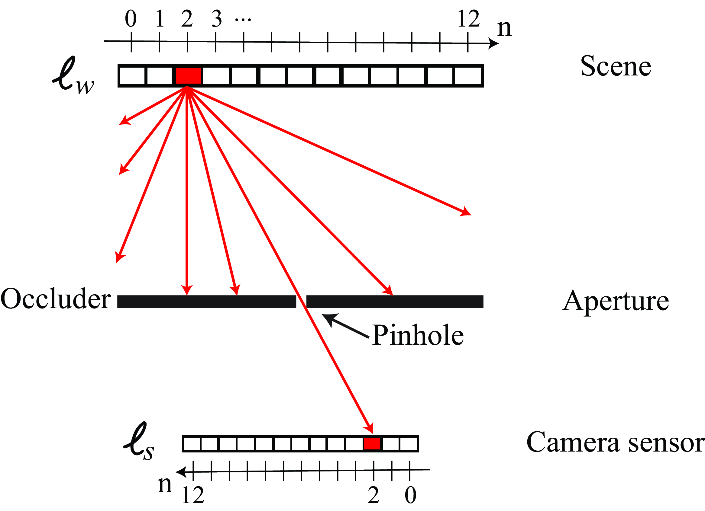
Let the light intensities in the world be represented by a column vector, \(\boldsymbol\ell_{\texttt{w}}\). The value of the \(n\)-th component of \(\boldsymbol\ell_{\texttt{w}}\) gives the intensity of the light at position \(n\), heading in the direction of the camera. There are a few more things to notice in Figure 7.1. The first one is that the axis in the camera sensor is reversed, consistent with Figure 5.8. The value \(n\) corresponds to image coordinates and the units are pixels. The second is that we are modeling the scene as being a line with varying albedos at a fixed depth from the camera. If the scene had a more complex spatial structure we would have to use the light field in order to use the same linear algebra that we will use in this chapter to model cameras. We will use light fields in Chapter 45.
In this chapter we will approximate the input light by a discrete and finite set of light rays instead of a continuous wave. This approximation allow us to use linear algebra to describe the imaging process.
7.3 Cameras as Linear Systems
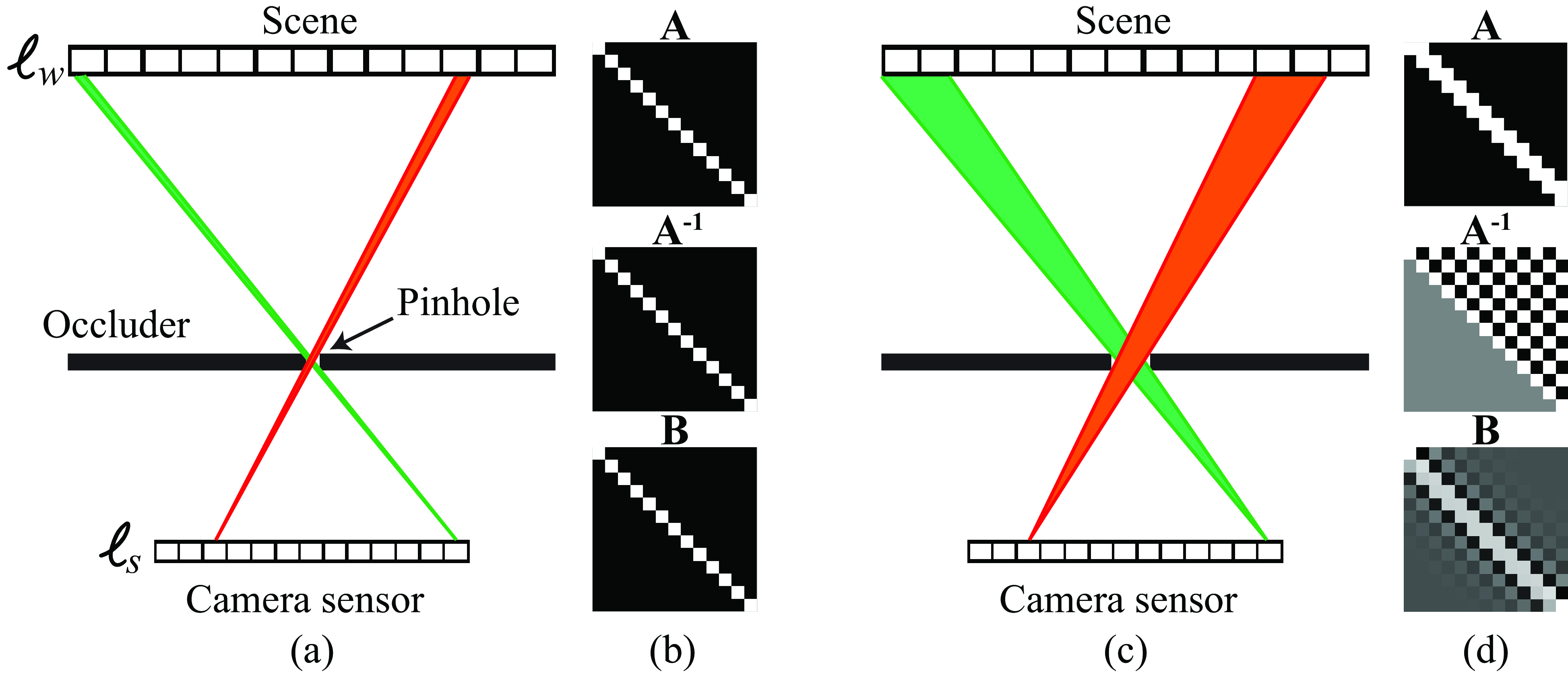
As shown in Figure 7.2 (a), the sensor is 1D and the scene lives in flatland. Let the sensor measurements be \(\boldsymbol\ell_{\texttt{s}}\) and the unknown scene be \(\boldsymbol\ell_{\texttt{w}}\). If the camera sensors respond linearly to the light intensity at each sensor, their measurements, \(\boldsymbol\ell_{\texttt{s}}\), will be some linear combination, given by the matrix, \(\mathbf{A}\), of the light intensities: \[ \boldsymbol\ell_{\texttt{s}} = \mathbf{A} \boldsymbol\ell_{\texttt{w}} \tag{7.1}\]
We represent the camera by matrix \(\mathbf{A}\). For the case of a pinhole camera, and assuming 13 pixel sensor observations, the camera matrix is just a 13×13 identity matrix, depicted in Figure 7.2 (b), as each sensor depends only on the value of a single scene element. For the case of conventional lens and pinhole cameras, where the observed intensities, \(\boldsymbol\ell_{\texttt{s}}\), are an image of the reflected intensities in the scene, \(\boldsymbol\ell_{\texttt{w}}\), then \(\mathbf{A}\) is approximately an identity matrix. For more general cameras, \(\mathbf{A}\) may be very different from an identity matrix, and we will need to estimate \(\boldsymbol\ell_{\texttt{w}}\) from \(\boldsymbol\ell_{\texttt{s}}\).
In the presence of noise, there may not be a solution \(\boldsymbol\ell_{\texttt{w}}\) that exactly satisfies ast squares sense. In most cases, \(\mathbf{A}\) is either not invertible, or is poorly conditioned. It is often useful to introduce a regularizr, an additional term in the objective function to. be minimized [1]. If the regularizaion term favors a smallworld \(\boldsymbol\ell_{\texttt{world}}\), then the objective term to minimize, \(E\), could be \[E = \lVert \boldsymbol\ell_{\texttt{s}}- \mathbf{A} \boldsymbol\ell_{\texttt{w}}\rVert ^2 + \lambda \lVert \boldsymbol\ell_{\texttt{w}}\rVert ^2 \tag{7.2}\]
The regularization parameter, \(\lambda\), determines the trade-off between explaining the observations and satisfying the regularization term.
Setting the derivative of Equation 7.2 of the vector \(\boldsymbol\ell_{\texttt{w}}\) equal to zero, we have \[ \begin{align} 0 &= \bigtriangledown_{\boldsymbol\ell_{\texttt{w}}} \lVert \boldsymbol\ell_{\texttt{s}}- \mathbf{A} \boldsymbol\ell_{\texttt{w}}\rVert ^2 + \bigtriangledown_{\boldsymbol\ell_{\texttt{w}}} \lambda \lVert \boldsymbol\ell_{\texttt{w}}\rVert ^2 \\ &= \mathbf{A}^T \mathbf{A} \boldsymbol\ell_{\texttt{w}}- \mathbf{A}^T \boldsymbol\ell_{\texttt{s}}+ \lambda \boldsymbol\ell_{\texttt{w}} \end{align} \tag{7.3}\] or
\[\boldsymbol\ell_{\texttt{w}}= (\mathbf{A}^T \mathbf{A} + \lambda \mathbf{I})^{-1}\mathbf{A}^T \boldsymbol\ell_{\texttt{s}} \tag{7.4}\]
Where the matrix \(\mathbf{B}=(\mathbf{A}^T \mathbf{A} + \lambda \mathbf{I})^{-1} \mathbf{A}^T\) is the regularized inverse of the imaging matrix \(\mathbf{A}\).
Next, consider the case of a wide aperture pinhole camera, shown in Figure 7.2 (c). If a single pixel in the sensor plane covers exactly two positions of the scene intensities, then the geometry is as shown in Figure 7.2 (c). Figure 7.2 (d) also shows the imaging matrix, \(\mathbf{A}\), its invere, \(\mathbf{A}^{-1}\), and the regularized inverse of the imaging matrix, which will usually give image reconstructions with fewer artifacts as it is less sensitive to noise. Note that \(\mathbf{A}^{-1}\) contains lots of fast changes that will make the result very sensitive to noise in the observation. The regularized matrix, \(\mathbf{B}\), shown in the bottom row of Figure 7.2 (d), is better behaved.
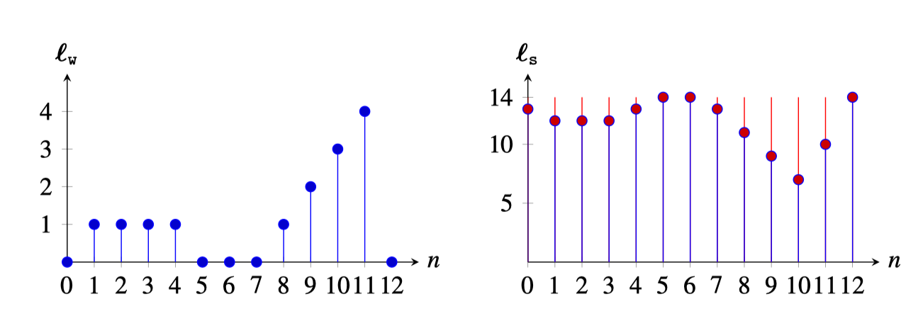
The following plot Figure 7.3 shows an example of an input 1D signal, \({\boldsymbol\ell_{\texttt{w}}}\), and the output of the 2-pixel wide pinhole camera, \({\boldsymbol\ell_{\texttt{s}}}\).
The output is obtained by multiplying the input vector by the matrix \(\mathbf{A}\) shown in he results of adding up two consecutive input values. The output is nearly identical to the input signal but with a larger magnitude and a bit smoother.
7.4 More General Imagers
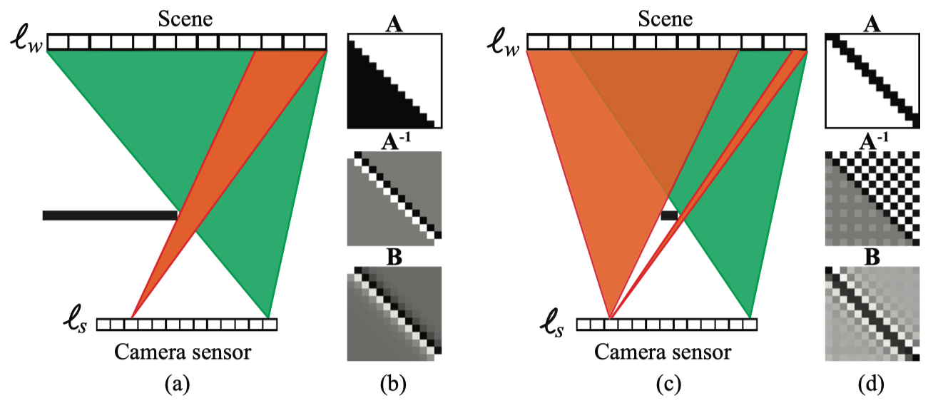
Many different optical systems can form cameras and the linear analysis described before can be used to characterize the imaging process. Even a simple edge will do. Figure 7.4 shows two non traditional imaging systems that we will analyze in this section.
7.4.1 Edge Camera
Consider the example of s to an edge camera. This is not a traditional pinhole camera; instead light is blocked only on one side.
For this camera, the imaging matrix and its inverse are as follows:
\[\mathbf{A} = \left[ \begin{array}{cccccc} 1 & 1 & 1 & 1 & \dots & 1 \\ 0 & 1 & 1 & 1 & ~ & 1 \\ 0 & 0 & 1 & 1 & ~ & 1 \\ 0 & 0 & 0 & 1 & ~ & 1 \\ \vdots & ~ & ~ & ~ & \ddots & ~ \\ 0 & 0 & 0 & 0 & ~ & 1 \end{array} \right], \mathbf{A}^{-1} = \left[ \begin{array}{cccccc} 1 & -1 & 0 & 0 & \dots & 0 \\ 0 & 1 & -1 & 0 & ~ & 0 \\ 0 & 0 & 1 & -1 & ~ & 0 \\ 0 & 0 & 0 & 1 & ~ & 0 \\ \vdots & ~ & ~ & ~ & \ddots & ~ \\ 0 & 0 & 0 & 0 & ~ & 1 \end{array} \right] \tag{7.5}\]
If we consider the same input as in the pinhole camera example in the previous section, the output signal for the corner camera will look like Figure 7.5:
The output now looks very different than that of a pinhole camera. In the pinhole camera, the output is very similar to the input. This is not the case here where the output looks like the integral of the input (reversed along the horizontal axis). Note that the first value of \(\boldsymbol\ell_{\texttt{s}}\) is equal to the sum of all the values of \(\boldsymbol\ell_{\texttt{w}}\): \[\ell_{\texttt{s}}\left[0 \right] = \sum_{n=0}^{12} \ell_{\texttt{w}}\left[n \right]\]
Figure 7.4 (b) illustrates the imaging matrix, \(\mathbf{A}\), and reconstruction matrices for the imager of Equation 7.5. You can think of this imager as computing an integral of the input signal. Therefore, its inverse looks like a derivative. The regularized inverse looks like a blurred derivative (we will talk more about blurred derivatives in Chapter 18).
7.4.2 Pinspeck Camera
Figure 7.4 (c) shows another nontraditional imager. Now, instead of a pinhole we have an occluder. The occluder blocks part of the light (complementary to the large-hole pinhole camera shown in Figure 7.4 (c)). What the camera sensor records is the shadow of the occluder. We can write the imaging matrix \(\mathbf{A}\), which corresponds to 1-\(\mathbf{A}_{pinhole}\) as shown in Figure 7.2 (d). Figure 7.4 (d) also shows its inverse and the regularized inverse. This camera is called a pinspeck camera [2], [3] and has also been used in practice.
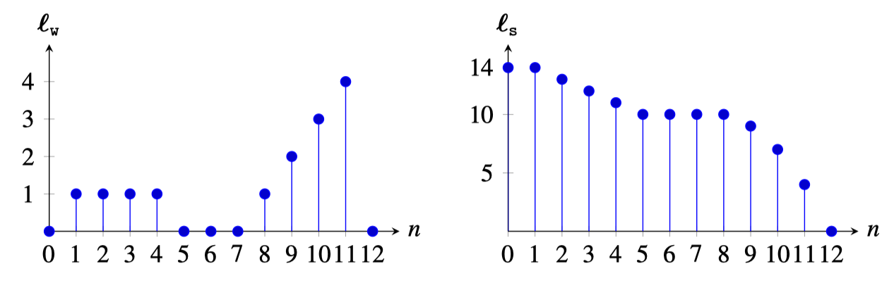
In the example of Figure 7.4 (c), the occluder has the size of the wide pinhole from Figure 7.2 (c). The following plots show Figure 7.6 (left), the input scene (same as in the previous examples), and Figure 7.6 (right), the output recorded by the camera sensor of the pinspeck camera.
The output is now a signal with a wide dynamic range (a max value of 14, which correspond to the sum of the values in \(\boldsymbol\ell_{\texttt{w}}\)) and with fluctuations due to the shadow of the occluder on the camera sensor. If there was no occluder, then the output would be a constant signal of value 14. In red we show the effect of the shadow, which is the light missing because of the presence of the occluder. You can see how the missing signal is identical to the output of the two-pixel wide pinhole camera but reversed in sign.
7.4.3 Corner Camera
To show a real-world example of a more general imager, let us consider the corner camera [4]. This is similar to the edge camera of Equation 7.5 and Figure 7.4, but with slightly more complicated geometry. As shown in Figure 7.7 (a), a vertical edge partially blocks a scene from view, creating intensity variations on the ground, observable by viewing those intensity variations from around the corner.
In practice, we will subtract a mean image from our observations of the ground plane, so in the rendering equation below, we will only consider components of the scene that may change over time, under the assumption that what we want to image behind the corner (e.g., a person) is moving. We will call these intensities \(S(\phi, \theta)\) (S for the subject), where \(\phi\) measures vertical inclination and \(\theta\) measures azimuthal angle, relative to the position where the vertical edge intersects the ground plane.
Integrating the light intensities falling on the ground plane, the observed intensities on the ground will be \(\boldsymbol\ell_{\texttt{ground}}(r, \theta)\), where the polar coordinates \(r\) and \(\theta\) are measured with respect to the corner. Assuming Lambertian diffuse reflection from the ground plane, we have for the observed intensities \(\boldsymbol\ell_{\texttt{ground}}(r, \theta)\): \[ \boldsymbol\ell_{\texttt{ground}}(r, \theta) = \int_{\phi=0}^{\phi=\pi} \int_{\xi=0}^{\xi=\theta} \cos(\phi) S(\phi, \xi) \, \mathrm{d} \phi \, \mathrm{d} \xi, \tag{7.6}\]
where the \(\cos(\phi)\) term in the equation follows from the equation for surface reflection discussed in Equation 5.2.
The dependence of the observation, \(\boldsymbol\ell_{\texttt{ground}}\), on vertical variations in \(S(\phi, \theta)\) is very weak, just through the \(\cos(\phi)\) term. We can integrate over \(\phi\) first, to form the 1D signal, \(\ell_{\texttt{w}}(\xi)\):
\[\ell_{\texttt{w}}(\xi) = \int_{\phi=0}^{\phi=\pi} \cos(\phi) S(\phi, \xi) \mbox{d} \phi \tag{7.7}\]
Then, to a good approximation, Equation 7.6 has the form, \[\boldsymbol\ell_{\texttt{ground}}(r, \theta) \approx \int_{\xi=0}^{\xi=\theta} \ell_{\texttt{w}}(\xi) \mbox{d} \xi, \tag{7.8}\] where \(\ell_{\texttt{w}}(\xi)\) is a 1D image of the scene around the corner from the vertical edge.
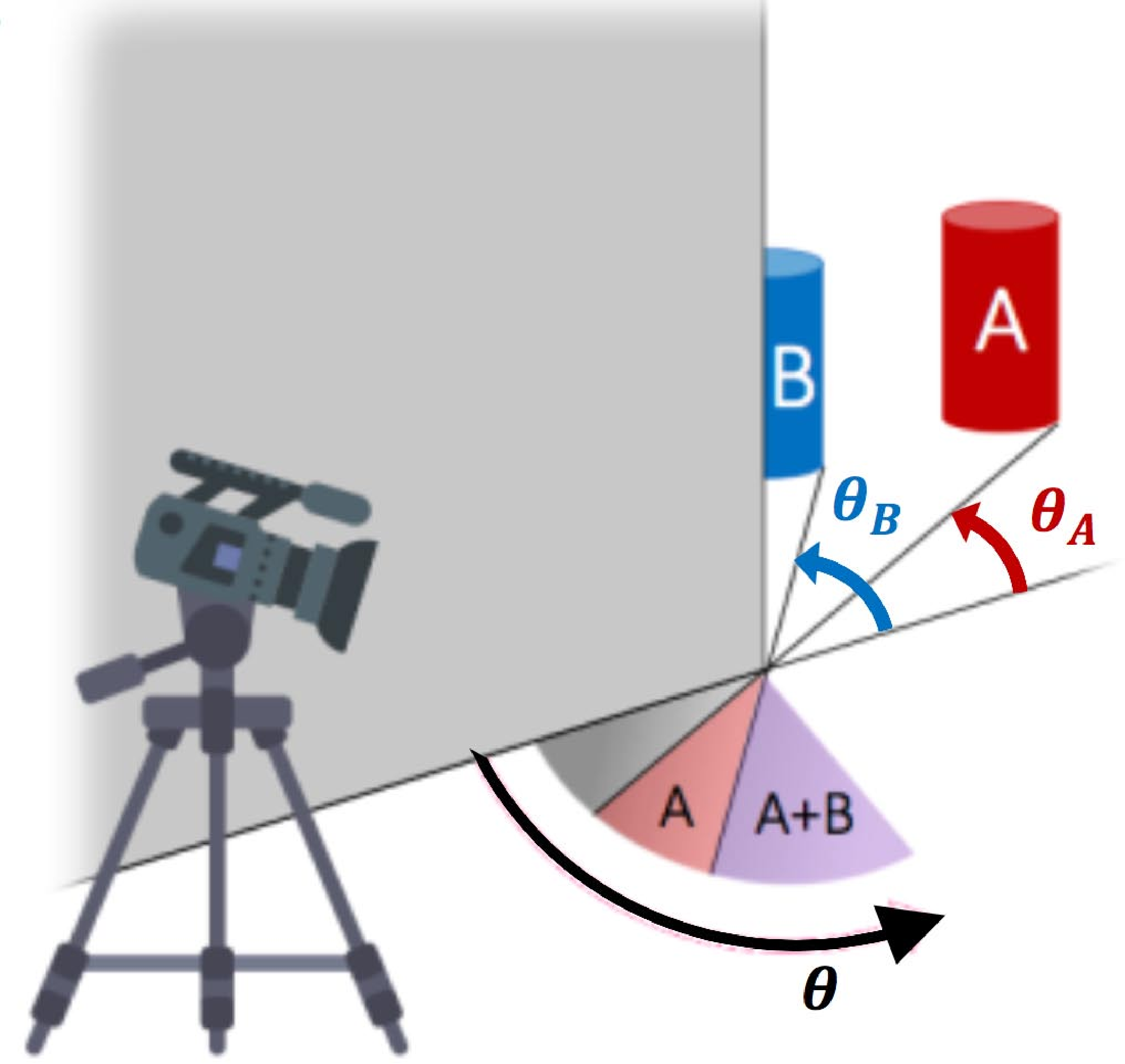
Figure 7.7 shows the corner camera geometry for a three-dimensional (3D) scene. Figure 7.7 (a) shows two objects, such as the cylinders labeled A and B, hidden behind a corner from a camera. Despite being behind the corner, they cause very small intensity differences in the ambient illumination falling on the ground, observable from the camera as a very small change in the light intensity reflecting from the ground. Can we reconstruct the scene hidden behind the corner using just the intensities observed on the ground? The image reconstruction operation is analogous to that for the edge camera of Figure 7.4: we subtract the reflected intensities observed at one orientation angle, say \(\theta_A\) from those observed at another, say \(\theta_B\).
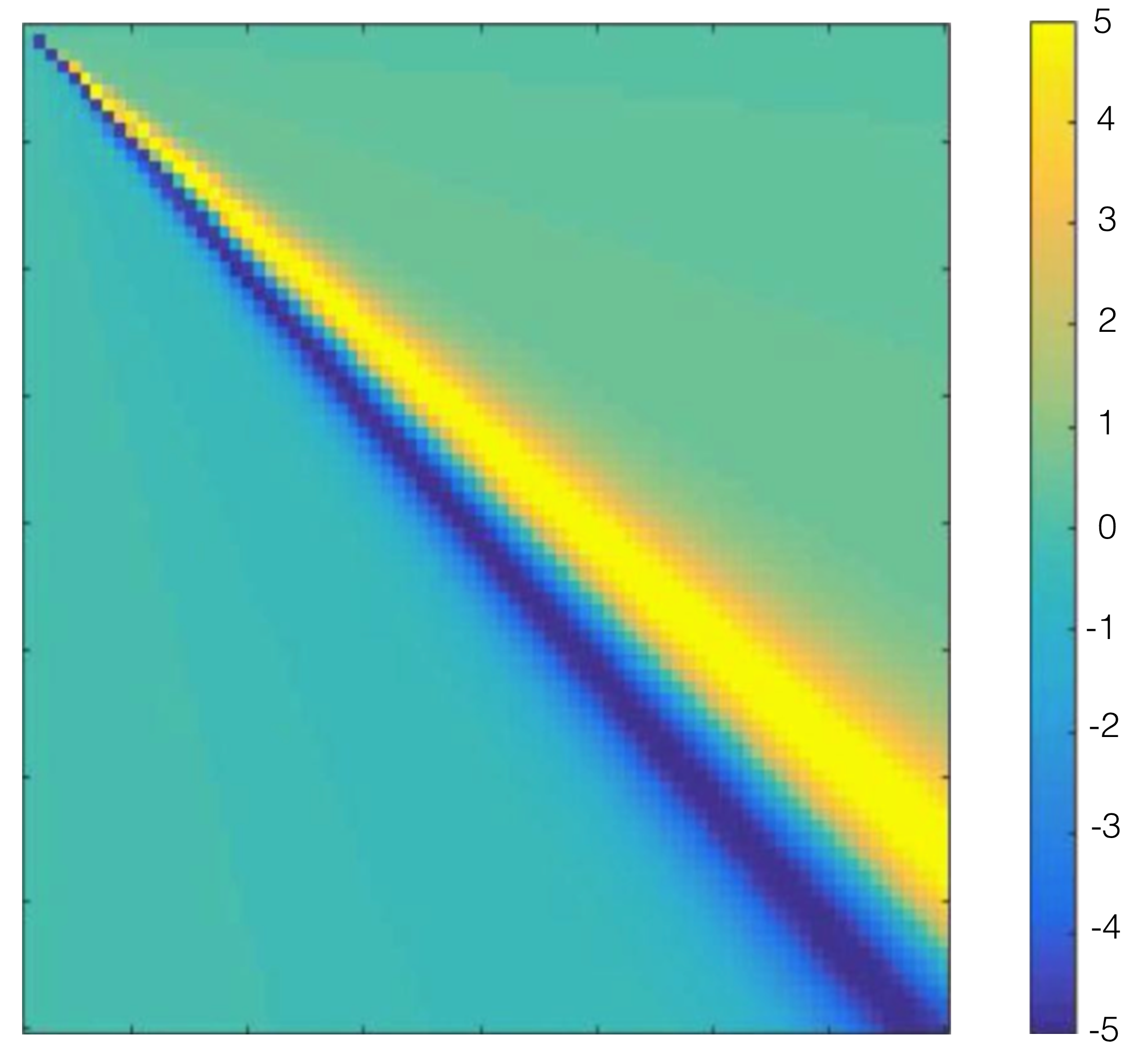
If we sample Equation 7.8 in its continuous variables, we can write it in the form \(\boldsymbol\ell_{\texttt{ground}} = \mathbf{A} \boldsymbol\ell_{\texttt{w}}\). Solving Equation 7.4 for the multiplier to apply to \(\boldsymbol\ell_{\texttt{ground}}\) to estimate \(\boldsymbol\ell_{\texttt{w}}\) yields the form shown in Figure 7.7 (b). Figure 7.7 (b) shows the spatial mask to be multiplied by the observed reflected ground image, with the result summed over all spatial pixels in order to estimate the light coming from around the corner at one particular orientation angle relative to the corner, in this case approximately 45 degrees. We see that the way to read the 1D signal from the ground plane is to take a derivative with respect to angle. This makes intuitive sense, as the light intensities on the ground integrate all the light up to the angle of the vertical edge. To find the 1D signal at the angle of the edge, we ask, “What does one pie-shaped ray from the wall see that the pie-shaped ray next to it doesn’t see?”
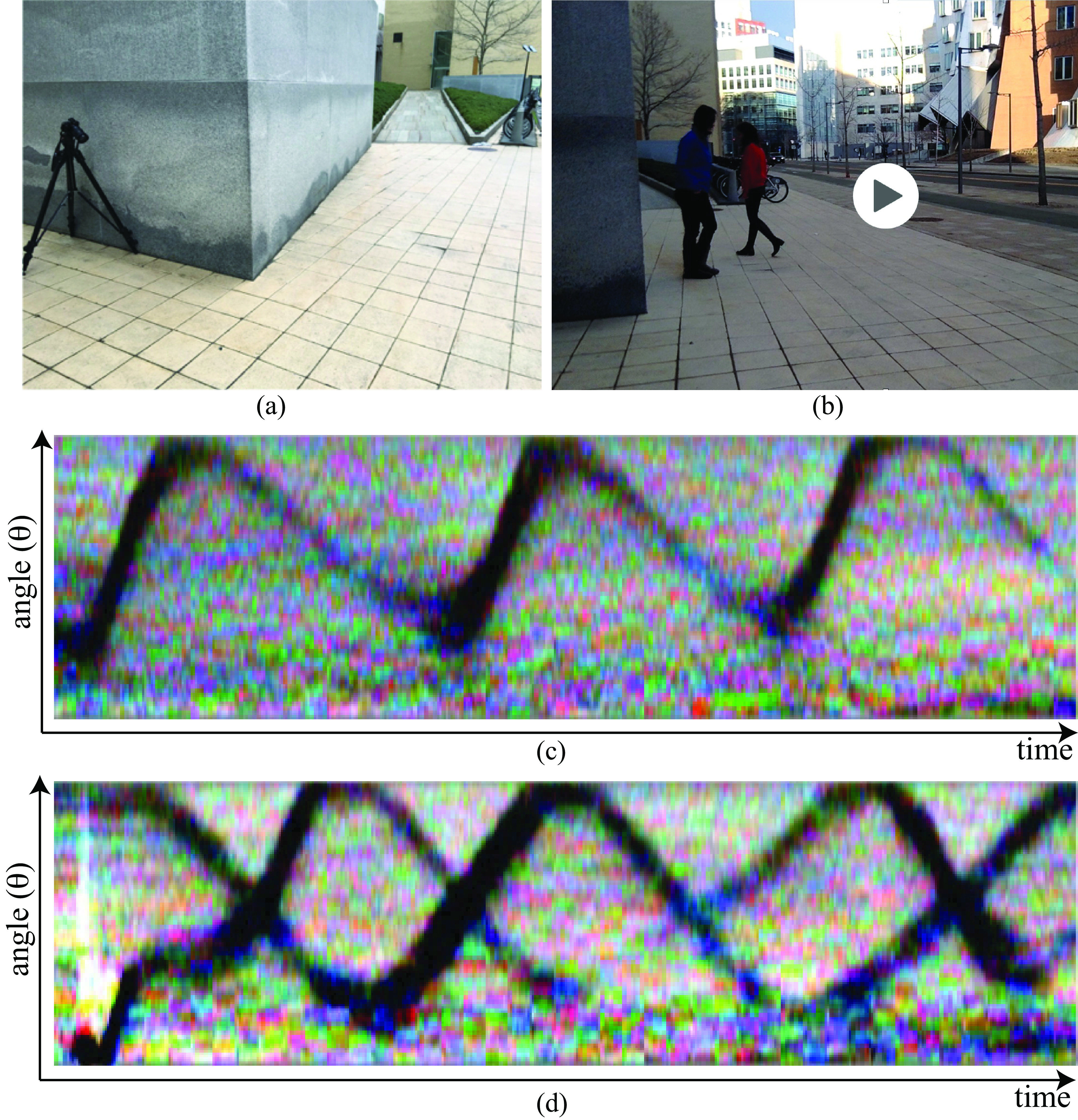
It can be shown [4] that the image intensities from around-the-corner scenes introduce a perturbation of about \(\frac{1}{1,000}\) to the light reflected from the ground from all sources. By averaging image intensities over the appropriate pie-shaped regions on the ground at the corner (Figure 7.7 (b)), one can extract a 1D image as a function of time from the scene around the corner. Figure 7.8 shows two 1D videos reconstructed from one (Figure 7.8 (a)) and two (Figure 7.8 (b)) people walking around the corner. By processing videos of very faint intensity changes on the ground, we can infer a 1D video of the scene around the corner. The image inversion formulas were derived using inversion methods very similar to Equation 7.4. The corner camera is just one of the many possible instantiations of a computational imaging system.
7.5 Concluding Remarks
Treating cameras as general linear systems allows for the machinery of linear algebra to be applied to camera design and processing. We reviewed several simple camera systems, including cameras utilizing pinholes, pinspecks, and edges to form images.