27 Statistical Image Models
27.1 Introduction
Building statistical models for images is an active area of research in which there has been remarkable progress. Understanding the world of images and finding rules that describe the pixel arrangements that are likely to be present in an image and which arrangements are not seems like a very challenging task. What we will see in this chapter is that some of the linear filters that we have seen in the previous chapters have remarkable properties when applied to images that allow us to put constraints on a model that aims to capture what real images look like.
First, we need to understand what we mean by a natural image. An image is a very high dimensional array of pixels \(\ell\left[n,m\right]\) and therefore, the space of all possible images is very large. Even if you consider very small thumbnails of just \(32\times32\) pixels and three color channels, with 8 bits per channel, there are more than \(10^{7,398}\) possible images. Of course, most of them will just be random noise. Figure 27.1 shows one image, with size \(32\times32\) color pixels, sampled from the set of natural images, and on typical example from the set of all images. A typical sample from the set of all images is \(32\times32\) pixels independently sampled from a uniform distribution.

As natural images are quite complex, researchers have used simple visual worlds that retain some of the important properties of natural images while allowing the development of analytic tools to characterize them. In the last decade, researchers have developed large neural networks that learned generative models of images and we discuss these models more in depth in Chapter 32. In this chapter we will focus on simpler image models as they will serve as motivation for some of the concepts that will be used later when describing generative models.
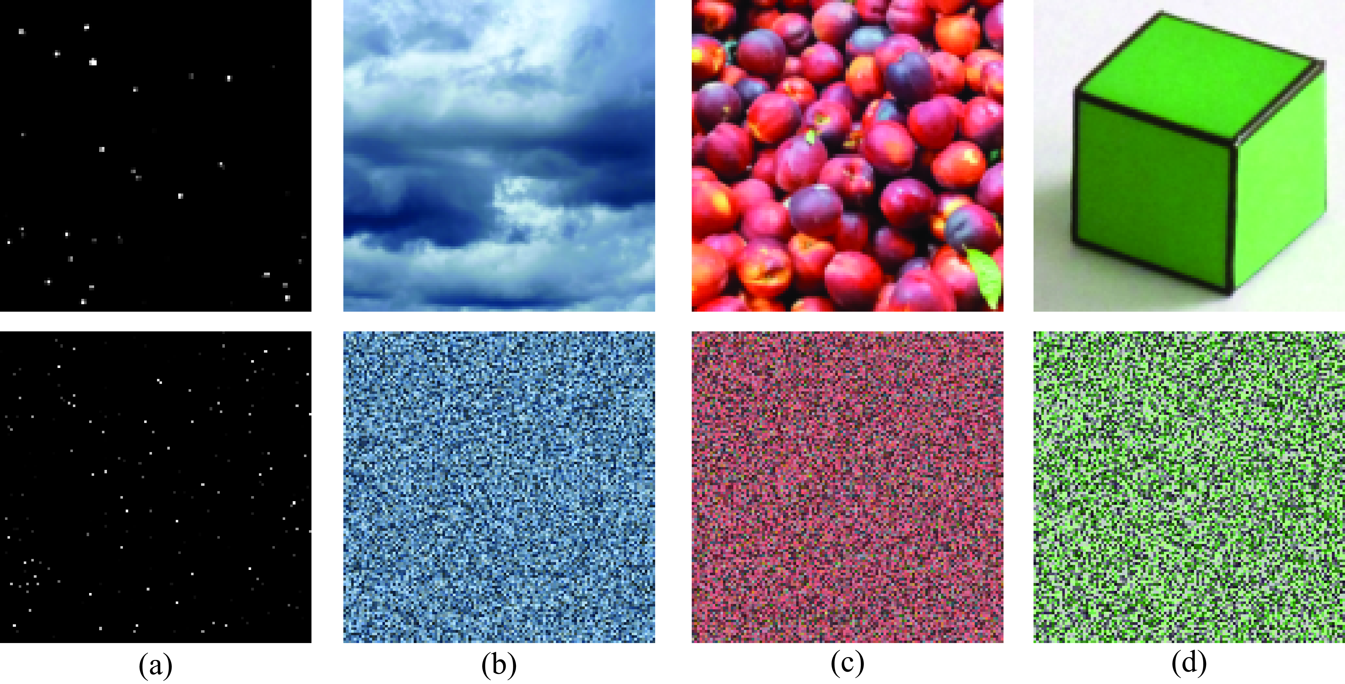
Figure 27.2 shows images that belong to different visual worlds. Each world has different visual characteristics. We can clearly differentiate images as belonging to any of these eight worlds, even if those visual worlds look like nothing we normally see when walking around. Explaining what makes images in the set of real images (Figure 27.2[h]) different to images in the other sets is not a simple task.
In this chapter we will talk, in some way or another, about all these visual worlds. The goal is to present a set of models that can be used to describe images with different properties. We will describe models that can be used to capture what makes each visual world unique. These models can be used to separate images into different causes, to remove noise from images, to predict the missing high-frequencies in blurry images, to fill in regions of missing image information due to occlusions, etc.

27.2 How Do We Tell Noise from Texture?
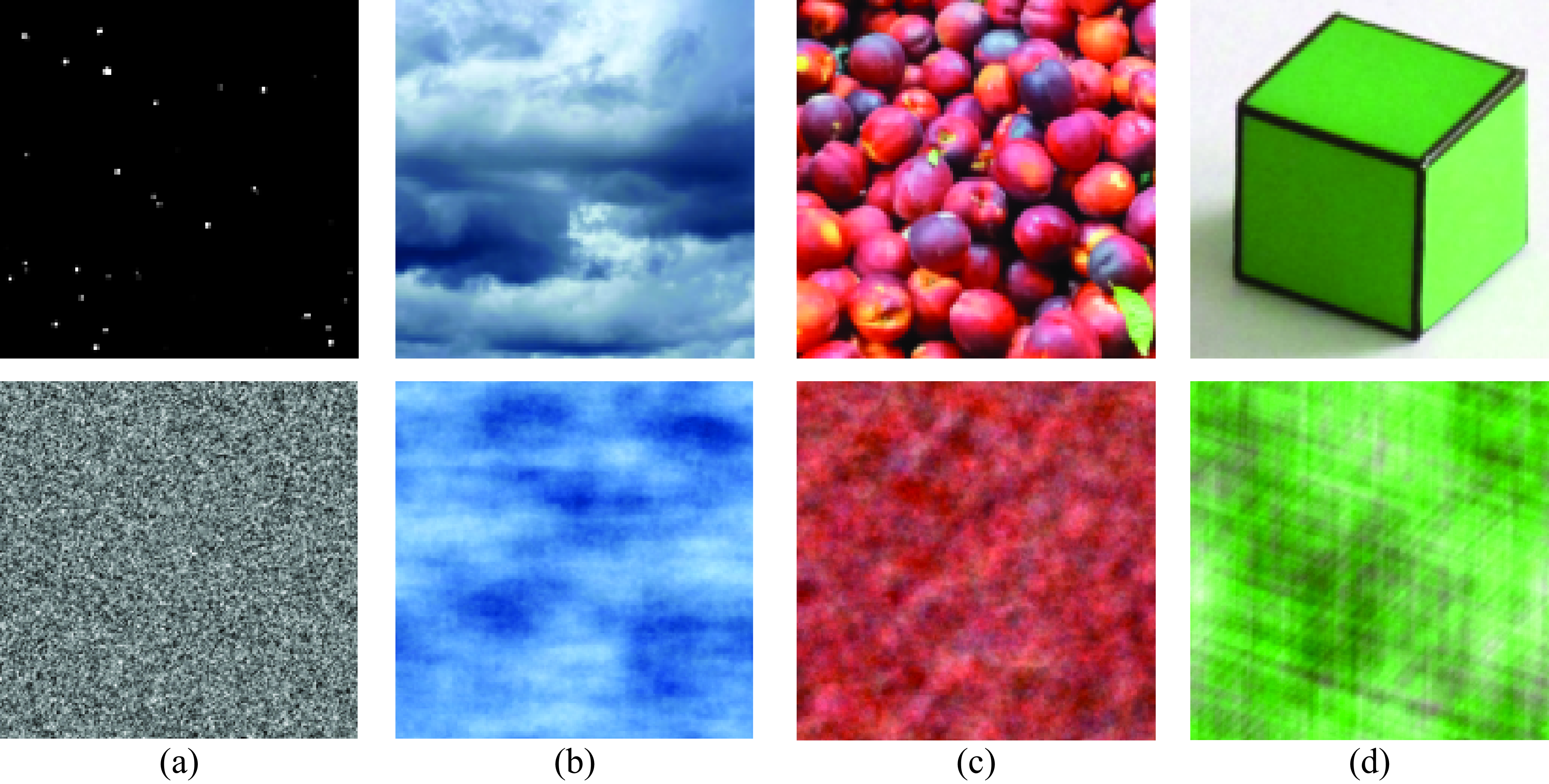
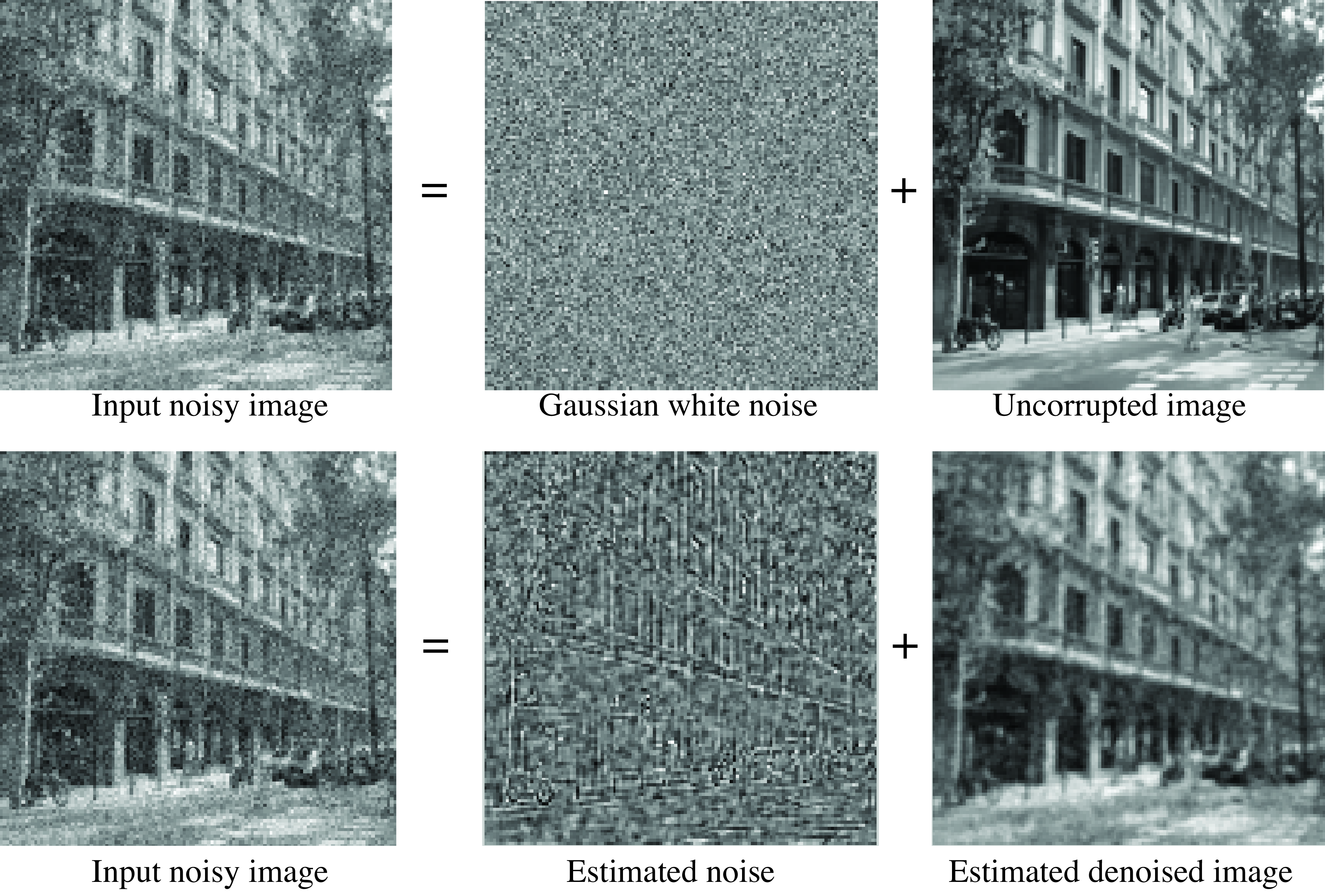
How do we tell noise from texture? Figure 27.3 shows two scenes: one image is corrupted with additive stationary noise added on top of the image, the other image contains one object textured with a pattern that looks like noise. Can you tell which one is which? Where is the noise? Is it in the image or in the world?
Stationary image noise is independent of the content of the scene, it is not affected by the object boundaries, it does not deform following the three-dimensional (3D) orientation of the surfaces, and it does not change frequency with distance between the camera and the scene. If the noise was really in the world, stationary noise would require a special noise distribution that conspires with the observer viewpoint to appear stationary.
Additive stationary noise is noise with statistical properties independent of location that is added to an observation. Check Section 27.5.2 for a more precise definition.
Noise is an independent process from the image content, and our visual system does not perceive noise as a strange form of paint. One important task in image processing is image denoising. Image denoising consists in removing the noise from an image automatically. This is equivalent to being able to separate the image into two components, one looking like a clean uncorrupted picture and the second image containing only noise. Statistical image models try to do this and more.
The original images from Figure 27.3
There is a significant interest in building image models that can represent whatever makes real photographs unique relative to, say, images that just contain noise. One way of building an image model is by having some procedural description, for instance a list of objects with locations, poses, and styles and a rendering engine, just as one would do when writing a program to generate CGI. One issue with this way of modeling images is that it will be hard to use it, and will require having an exhaustive list of all the things that we can find in the world. We will see later that the apparent explosion in complexity should not stop us. However, there is another way of building image models. In the rest of this chapter we will study a very different approach that consists of building statistical models of images that try to capture the properties of small image neighborhoods. Statistical models are also foundational in other disciplines such as natural language modeling. Here we will review models of images of increasing complexity, starting with the simplest possible neighborhood: the single pixel.
27.3 Independent Pixels
The simplest image model will consist in assuming that all pixels are independent and their intensity value is drawn from some stationary distribution (i.e., the distribution of pixel intensities is independent of the location in the image). We can then write the probability, \(p_{\theta}(\boldsymbol\ell)\), of an image, \(\ell[n,m]\) with size \(N \times M\), as follows: \[p_{\theta}(\boldsymbol\ell) = \prod_{n=1}^{N} \prod_{m=1}^{M} p_{\theta}\left(\ell[n,m] \right) \tag{27.1}\] We use \(p_{\theta}\) to denote a parameterized probability model. The vector \(\theta\) contains the parameters and can be fitted to data using maximum likelihood or other loss functions. We will see many variants of this probability model here and in the following chapters.
One way of assessing the accuracy of a statistical image model is to sample from the model and view the images it produces. This will require knowing the distribution \(p_{\theta}\left(\ell[n,m] \right)\).
What we can do is to take one image from one of the visual worlds that we described in the introduction, and then estimate the model \(p_{\theta}\left(\ell[n,m] \right)\), as illustrated in Figure 27.4.
In the case of discrete gray-scale images with 256 gray levels, we can represent the distribution \(p_{\theta}\) as vector of 256 values indicating the probability of each intensity value. In the case of considering color images with 256 levels on each channel (i.e., 8 bits per channel) we will have \(256^3\) bins in the color histogram.
The parameters, \(\theta\), of the distribution are those 256 (or \(256^3\) for color) values. If we are given a set of images, we can estimate the vector \(\theta\) as the average histogram of the images. We can also estimate the model from a single image. We can then sample new images based on equation (Equation 27.1). In order to sample a new image, we will sample each pixel independently using the intensity distribution given by the training set.
The procedure for four training images is shown in Figure 27.5. As illustrated in Figure 27.5, the process starts by computing the average color histogram for the four images. Then, we sample a new image by sampling every pixel from the multinomial defined by the \(p_{\theta}\).
In the multinomial model, the probability that the image in location \((n,m)\) has the value \(k\) is \(p_{\theta}(\ell [n,m] = k) = \theta_k\). In the case of color images, in this model, \(k\) will be one of the \(256^3\) possible color values.
Figure 27.6 shows four pairs of images with matched color histograms. We can see that this simplistic model is somewhat appropriate for pictures of stars (although star images can have a lot more structure), but it miserably fails in reproducing anything with any similarity (besides the overall color) to any of the other images. The failure of color histograms as a generative model of images should not be surprising as treating pixels as independent observations is clearly not how images work.
As a generative model of images, this model is very poor. However, this does not mean that image histograms are not important. Manipulating image histograms is a very useful operation. Given two images \(\boldsymbol\ell_1\) and \(\boldsymbol\ell_2\) with histograms \(\mathbf{h}_1\) and \(\mathbf{h}_2\), we look for a pixelwise transformation \(f\left(\ell[n,m] \right)\) so that the histogram of the transformed image, \(f\left(\ell_1 [n,m] \right)\), matches the histogram of \(\boldsymbol\ell_2\). There are many ways in which histograms can be transformed. One natural choice is a transformation that preserves the ordering of pixels intensities.
Figure 27.7 shows examples of spheres that are reflecting some complex ambient illumination. This is an example that illustrates the perceptual importance of simple histogram manipulations. The two spheres on the left are the two original images. The ones on the left are generated by modifying the image histograms to match the histogram of the opposite image. The figure shows that by simply changing the image histogram we can transform how we perceive the material of each sphere: from shiny to matte [1]. The sphere was first rendered with two illumination models: from a campus photograph (Figure 27.7 (a)), and from pink noise (Figure 27.7 (b)). Pink noise is random noise with a \(\frac{1}{|w_x^2+w_y^2|}\) power spectrum, where \(w_x\) and \(w_y\) are the spatial frequencies. In Figure 27.7 (c) and Figure 27.7 (d) the sphere histograms were swapped, creating a different sense of gloss in the sphere images. Note how by simply modifying the image histograms within the pixels of the sphere, the sphere seems to be made by a different type of material.
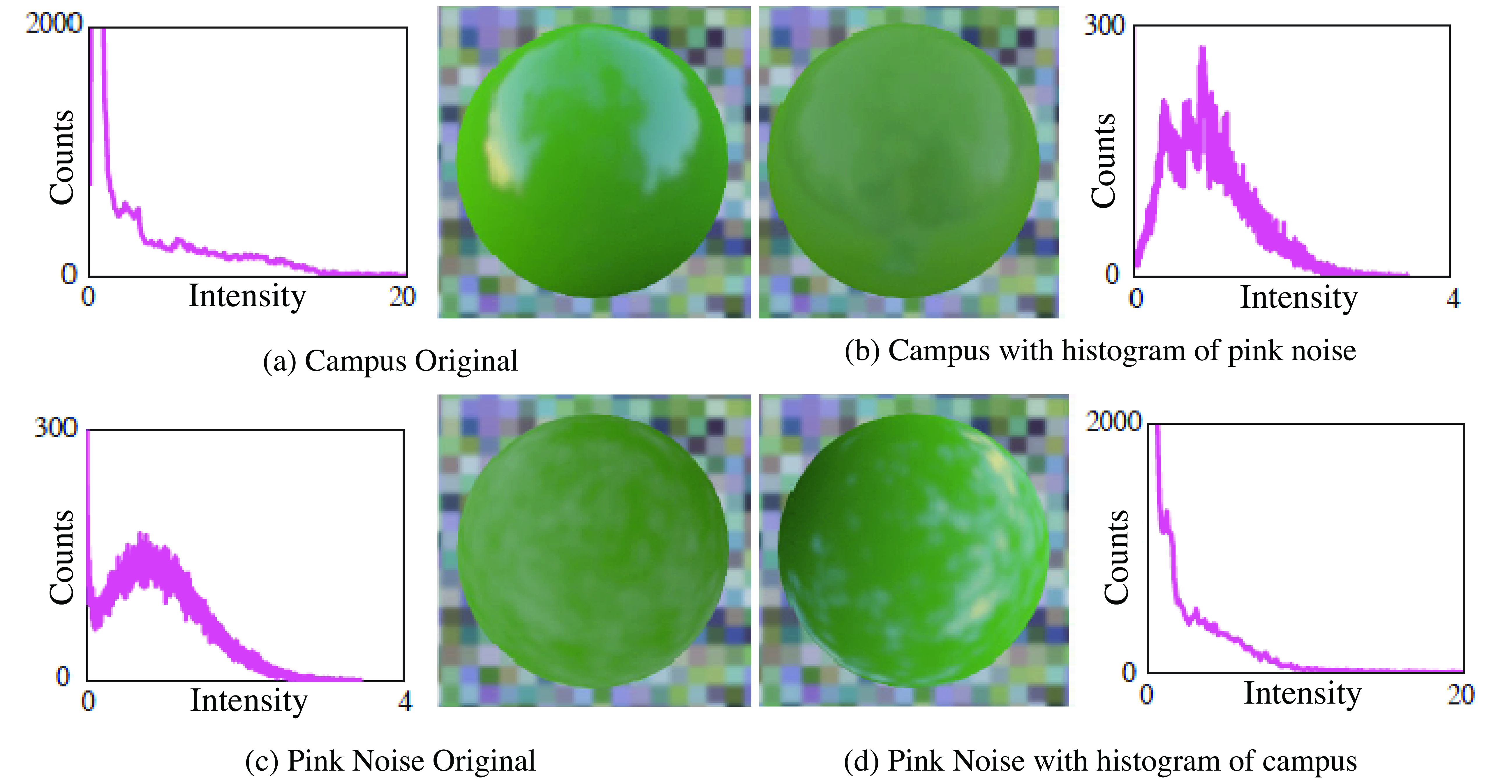
Image histograms carry useful information, but the histogram alone fails in capturing what makes images unique. We will need to build a more sophisticated image model.
27.4 Dead Leaves Model
In the quest to find what makes photographs of everyday scenes special, the next simplest image structure is a set of two pixels. Things get a lot more interesting now. If one plots the value of the intensity of one pixel as a function of the intensity value of the pixel nearby, the scatterplot produced by many pixel pairs (Figure 27.8) is concentrated on the identity line. As we look at the correlation between pixels that are farther away, the correlation value slowly decays. The correlation, \(C\), between two pixels separated by offsets of \(\Delta n\) and \(\Delta m\), is: \[C(\Delta n, \Delta m) = \rho \left( \ell[n+\Delta n,m+ \Delta m], \ell[n,m] \right) \tag{27.2}\] where \[\rho \left( a, b \right) = \frac{E \left( (a-\bar{a})( b- \bar{b}) \right)}{\sigma_a \sigma_b},\]where \(\sigma_a\) is the standard deviation of the variable \(a\), and \(\bar{a}\) is the mean of \(a\).
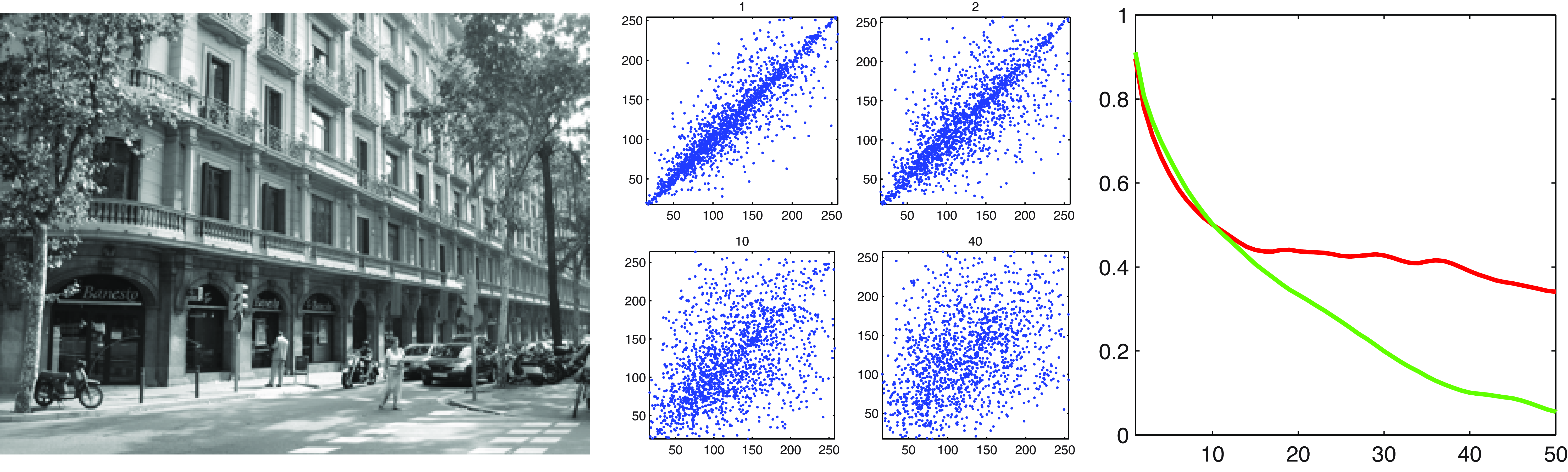
The behavior of this correlation function when computed on natural images is very different from the one we would observe if the correlation was computed over white noise images.
There have been many efforts to model the minimal set of assumptions needed in order to produce image-like random processes. The dead leaves model is a simplified image formation model that tries to approximate some of the properties observed for natural images. This model was introduced in the 1960s by Matheron [2] and popularized by Ruderman in the 90’s [3]. The model is better described by a procedure. An image is modeled as a set of shapes (dead leaves) that fall on a flat surface generating a random superposition (e.g., Figure 27.9).
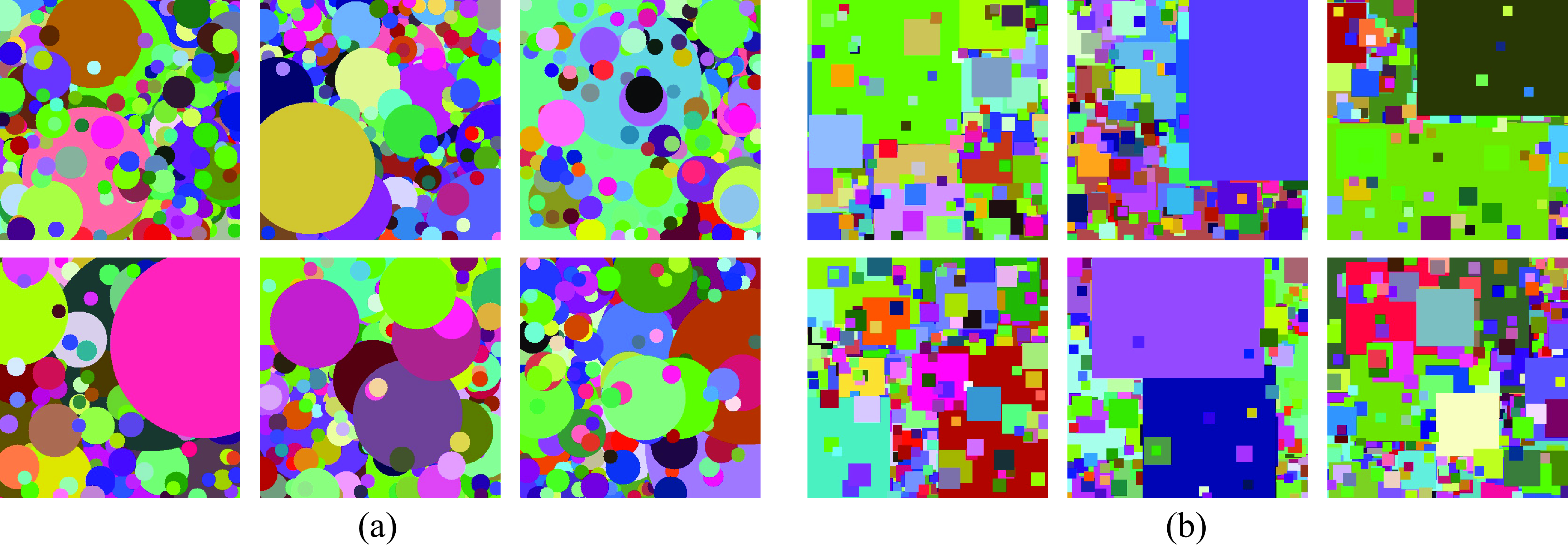
The dead leaves model produces very simple images that do not look realistic, but it is useful in explaining the distribution of albedos in natural images. This model is used by the Retinex algorithm [4] to separate an image into illumination and albedo variations, as we saw in Chapter 18.
27.4.1 The Power Spectrum of Natural Images
The correlation function from equation (Equation 27.2) is related to the magnitude of the Fourier transform of an image.
The Fourier transform of the autocorrelation of a signal is the square of magnitude of its Fourier Transform. The square of the magnitude of the FT, \(\lVert \mathscr{L}(u,v) \rVert ^2\), is the power spectrum of a signal.
Interestingly, the one remarkable property of most natural images is that if you take the 2D Fourier transform of an image, its magnitude falls off as a power law in frequency: \[\lVert \mathscr{L}(u,v) \rVert \simeq \frac{1}{ w ^ \alpha} \tag{27.3}\] where \(w\) denotes the radial spatial frequency (\(w = \sqrt{u + v}\)), \(\mathscr{L}(u,v)\) is the Fourier transform of the image \(\ell[n,m]\), and \(\alpha \simeq 1\). And this is true for all orientations (you can think of this as taking the Fourier transform and looking at the profile of a slice that passes by the origin).
The fact that most natural images follow equation (Equation 27.3) has been the focus of an extensive literature [5], [6], and it has been shown to be related to several properties of the early visual system [7], [8] which is adapted to process natural images. We will see in the next section how this model can be used to solve a number of image processing tasks.
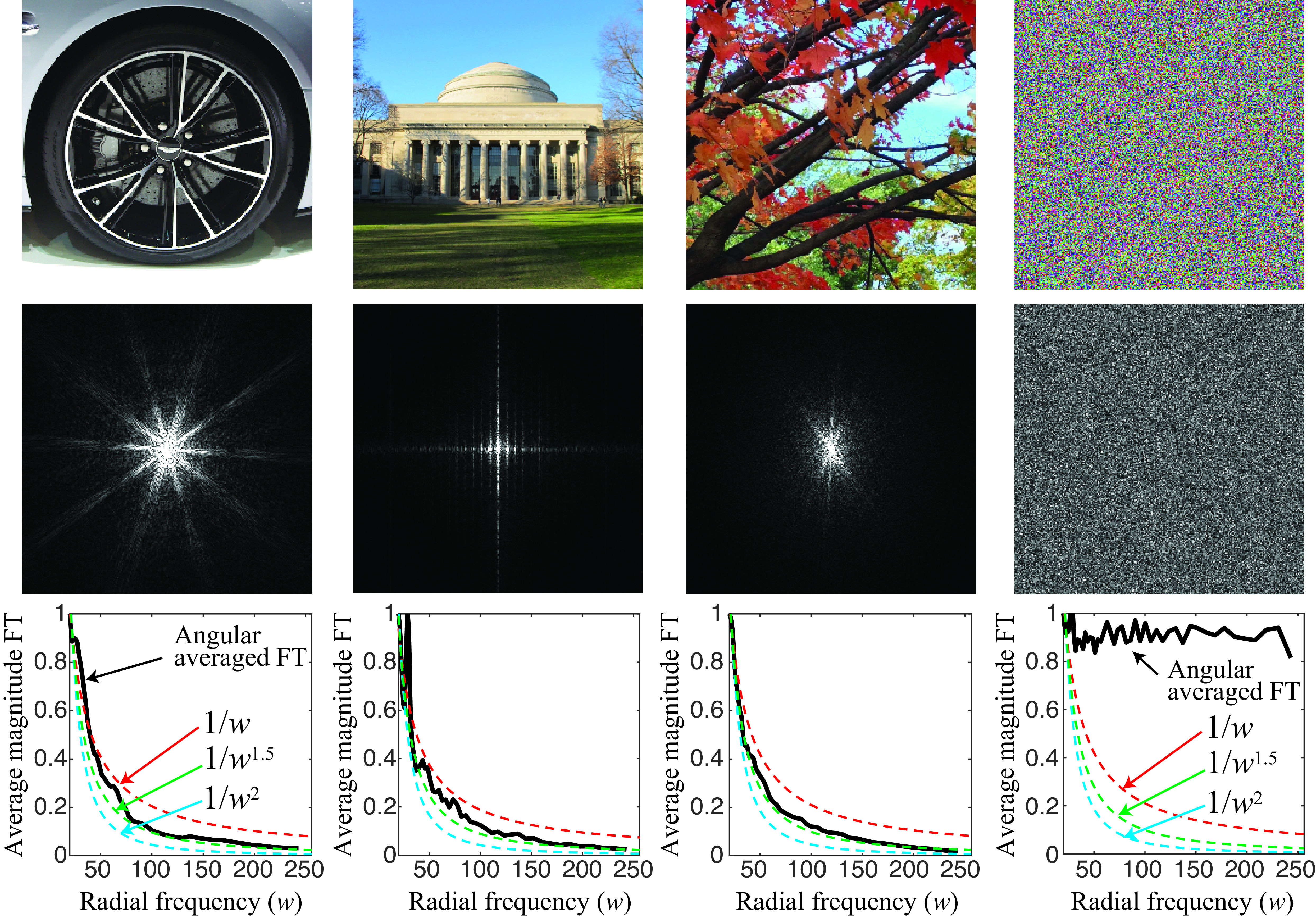
Figure 27.10 shows three natural images and the magnitude of their FT (middle row), and compares them to a random image where each pixel is independently sampled from a uniform distribution. The frequency \((0,0)\) lies in the middle of each FT. From the images in the middle row, we can see that the largest amplitudes concentrate in the low spatial frequencies for the natural images (we already discussed this in Chapter 16). However, the random image has similar spectral content at all frequencies. In order to better appreciate the particular decay in the spectral amplitude with frequency, we can express the FT using polar coordinates, then calculate the average magnitude of the FT by aggregating the values over all angular directions. The result is shown in the bottom row of Figure 27.10. The plot also shows three additional curves corresponding to \(1/w\), \(1/w^{1.5}\), and \(1/w^2\). The plots are normalized to start at 1. These images have size 512 \(\times\) 512. The frequency ranges used for the plot are \(w \in [20,256]\). As we can see from the middle row, there are differences on how spectral content is organized across orientations, but the decay along the radial frequency roughly follows a \(1/w^{1.5}\) decay in these examples. And these property is shared across the four images despite their very distinct appearance.
We will now use this observation to build a better statistical model of images than using pixel histograms as we described in Section 27.3.
27.5 The Gaussian Model
We want to write a statistical image model that takes into account the correlation statistics and the power spectrum of natural images (see [9] for a review). If the only constraint we have is the correlation function among image pixels, which means that among all the possible distributions, the one that has the maximum entropy (thus, imposing the fewest other constraints) is the Gaussian distribution: \[p(\boldsymbol\ell) \propto \exp \left(-\frac{1}{2} \boldsymbol\ell^\mathsf{T}{\bf C}^{-1} \boldsymbol\ell\right) \tag{27.4}\] where \({\bf C}\) is the covariance matrix of all the image pixels. Note that this model no longer assumes independence across pixels. It accounts for the correlation of intensity values between different pixels, as discussed in previous sections. This model is also related to studies that use principal component analysis to study the typical components of natural images [10].
For stationary signals, the covariance matrix \({\bf C}\) has a circulant structure (assuming a tiling of the image) and can be diagonalized using the Fourier transform. The eigenvalues of the diagonal matrix correspond to the power (squared magnitude) of the frequency components of the Fourier transform. This is, the matrix \({\bf C}\) can be written as \({\bf C} = {\bf F}{\bf D}{\bf F}^\mathsf{T}\). Where \({\bf F}\) is the matrix that contains the Fourier basis, as seen in Chapter 16, and the diagonal matrix \({\bf D}\) has, along the diagonal, the values \(1/ w ^\alpha\) for all radial frequencies \(w\). The value of \(\alpha\) can be set to a fix value of 1.5.
27.5.1 Sampling Images
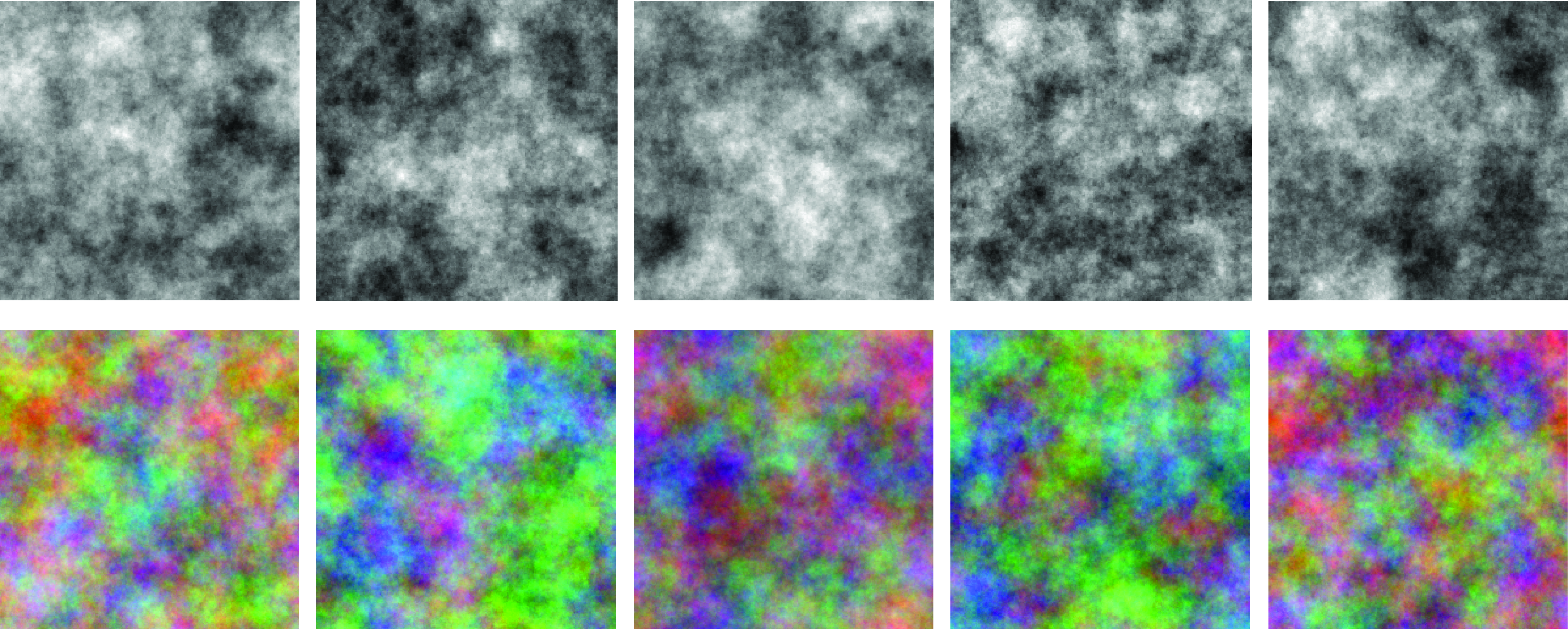
Once a distribution is defined, we can use it to sample new images. First we need to specify the parameters of the distribution. In this case, we need to specify the covariance matrix \({\bf C}\). Figure 27.11 shows the results of sampling images using the \(1/ w^\alpha\) model to fill the diagonal values of the matrix \({\bf D}\). These images are generated by making an image with a random phase and with a magnitude of the power spectrum following \(1/(1+w ^\alpha)\) with \(\alpha=1.5\). We add 1 to the denominator term to avoid division by zero. The bottom row of Figure 27.11 generates color images by sampling each color channel independently.
We can also sample new images by matching the parameter of individual natural images. Figure 27.12 shows four examples. To process color images, we first look for a color space that decorrelates color information for each image. This can be done by applying principal component analysis (PCA) to the three color channels. This results in a \(3 \times 3\) matrix that will produce three new channels that are decorrelated. Then, for each channel, we compute the FT and keep the magnitude and replace the phase with random noise. We finally compute the new generated imaged by doing the inverse FT and applying the inverse of the PCA matrix in order to return to the original color space. This results in images that keep a similar color distribution than the inputs.
As shown in Figure 27.12, when fitting the Gaussian model to different real images, and then sampling from it, the result is always an image that looks like cloudy noise regardless of the image content. However, a few attributes of the original image are preserved including the size of the details present in the image and the dominant orientations.
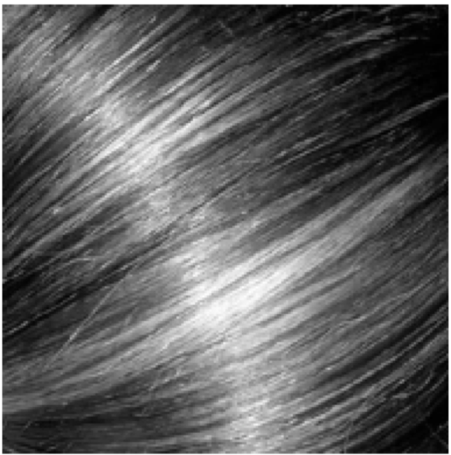
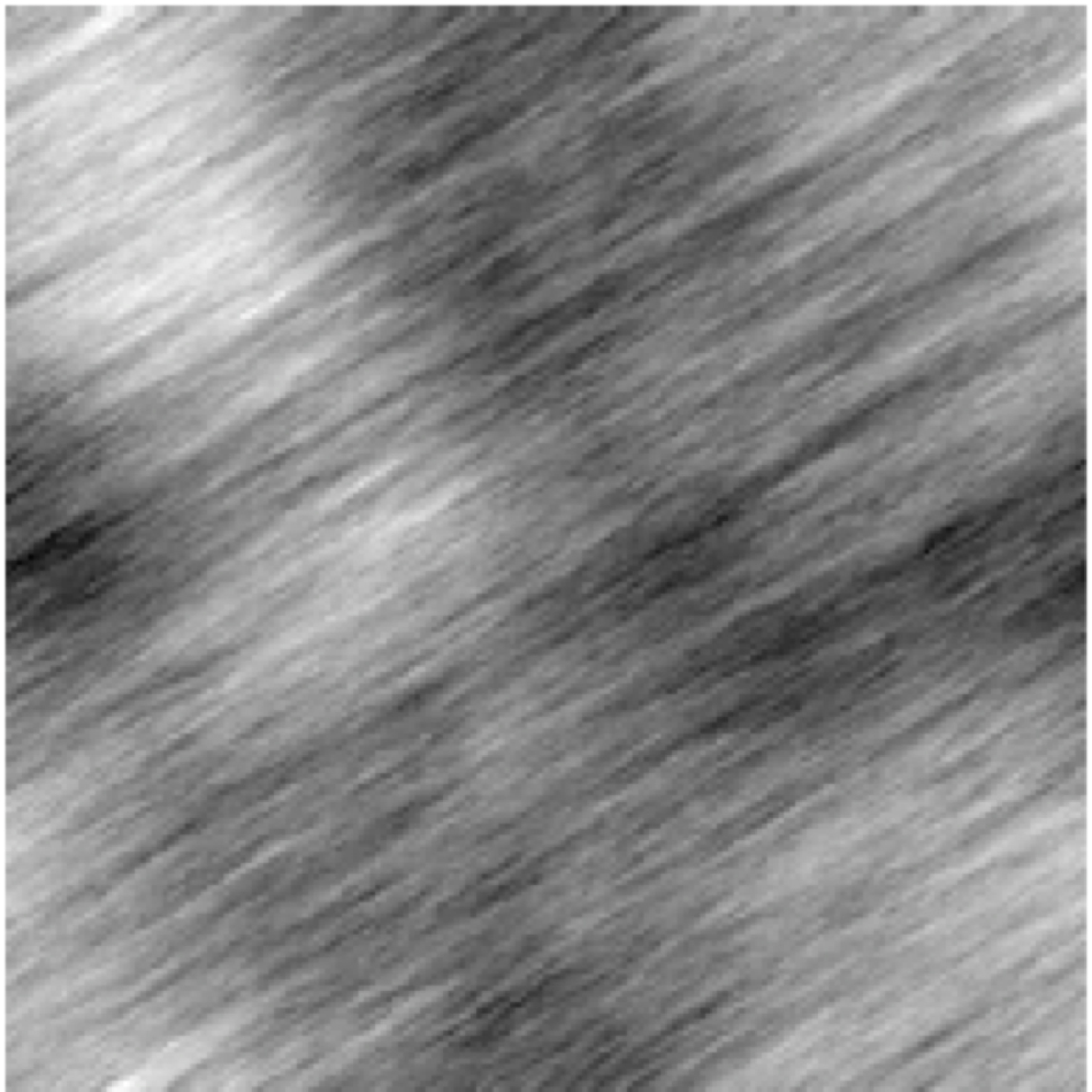
Figure 27.13 shows an example image where the sample from its Gaussian model produces a similar image, due to the strong oriented pattern present in the image. In this example, the input image is mostly one-dimensional (1D) as most of the variations occur across one orientation being constant along the perpendicular direction. This structure can be captured by the magnitude of the Fourier transform of the image.
The Gaussian image model, despite being very simple, can be used to study some image processing tasks, including image denoising, which we will discuss next.
Devising processes that generate realistic textures has a long history and many applications in the movie industry. One example is Perlin noise developed by Ken Perlin in 1985. In the rest of this book, we will study in depth the image generation problem when talking about generative models.
27.5.2 Image Denoising under the Gaussian Model: Wiener Filter
As an example of how to use image priors for vision tasks, we will study how to do image denoising using the prior on the structure of the correlation of natural images. In this problem, we observe a noisy image \(\boldsymbol\ell_g\) corrupted with white Gaussian noise: \[\ell_g[n, m] = \ell[n, m] + g[n, m]\] The goal is to recover the uncorrupted image \(\ell[n,m]\). The noise \(g[m, n]\) is white Gaussian noise with variance \(\sigma_g^2\). The denoising problem can be formulated as finding the \(\ell[n,m]\) that maximizes the probability of the uncorrupted image, \(\boldsymbol\ell_g\), called the maximum a posteriori, or MAP, estimate: \[\max_{\boldsymbol\ell} p(\boldsymbol\ell\bigm | \boldsymbol\ell_g)\] In these equations we write the image as a column vector \(\boldsymbol\ell\). This posterior density can be written as: \[\max_{\boldsymbol\ell} p({\boldsymbol\ell} \bigm | {\boldsymbol\ell}_g) = \max_{\boldsymbol\ell} p({\boldsymbol\ell}_g \bigm | {\boldsymbol\ell}) p({\boldsymbol\ell})\] where the likelihood and prior functions are: \[\begin{aligned} p({\boldsymbol\ell}_g \bigm | {\boldsymbol\ell}) & \propto \exp( - \left| {\boldsymbol\ell}_g - {\boldsymbol\ell} \right| ^2 / \sigma_g^2) \\ p({\boldsymbol\ell}) & \propto \exp \left(-\frac{1}{2} {\boldsymbol\ell}^T {\bf C}^{-1} {\boldsymbol\ell} \right) \end{aligned}\] The solution to this problem can be obtained in closed form: \[{\boldsymbol\ell} = {\bf C} \left( {\bf C} + \sigma_g^2 \mathbf{I} \right)^{-1} {\boldsymbol\ell}_g\] This is just a linear operation. It can also be written in the Fourier domain as: \[\mathscr{L}(v) = \frac{A/|v|^{2\alpha}}{A/|v|^{2\alpha} + \sigma_g^2} \mathscr{L}_g(v)\]
Figure 27.14 shows the result of using the Gaussian image model for image denoising. Although there is a certain amount of noise reduction, the result is far from satisfactory. The Gaussian image model fails to capture the properties that make a natural image look real.
27.6 The Wavelet Marginal Model
As we showed previously, sampling from a Gaussian prior model generates images of clouds. Although the Gaussian prior does not give any image zero probability (i.e., by sampling for a very long time it is not impossible to sample the Mona Lisa), the most typical images under this prior look like clouds.
The Gaussian model captures the fact that pixel values are correlated and that such correlation decreases with distance. However, it fails to capture other very important properties of images, such as flat regions, edges, and lines. Here, we extend the Gaussian model in two ways. (1) We will use localized filters instead of sinusoids (i.e., Fourier basis) that span the entire image, as in the power spectrum model used in the previous section. This helps to capture local structure such as lines and edges. (2) Instead of characterizing the outputs of those filters by a single number (e.g., the mean power), we measure the histogram shape of all the filter responses.
In the 1980s, a number of papers noticed a remarkable property of images: when filtering images with band-pass filters (i.e, image derivatives, Gabor filters, etc.) the output had a non-Gaussian distribution [11], [5]. Figure 27.15 shows the histogram of the input image and the histogram of the output of applying the filters \(\left[-1,1\right]\) and \(\left[-1,1\right]^\mathsf{T}\).
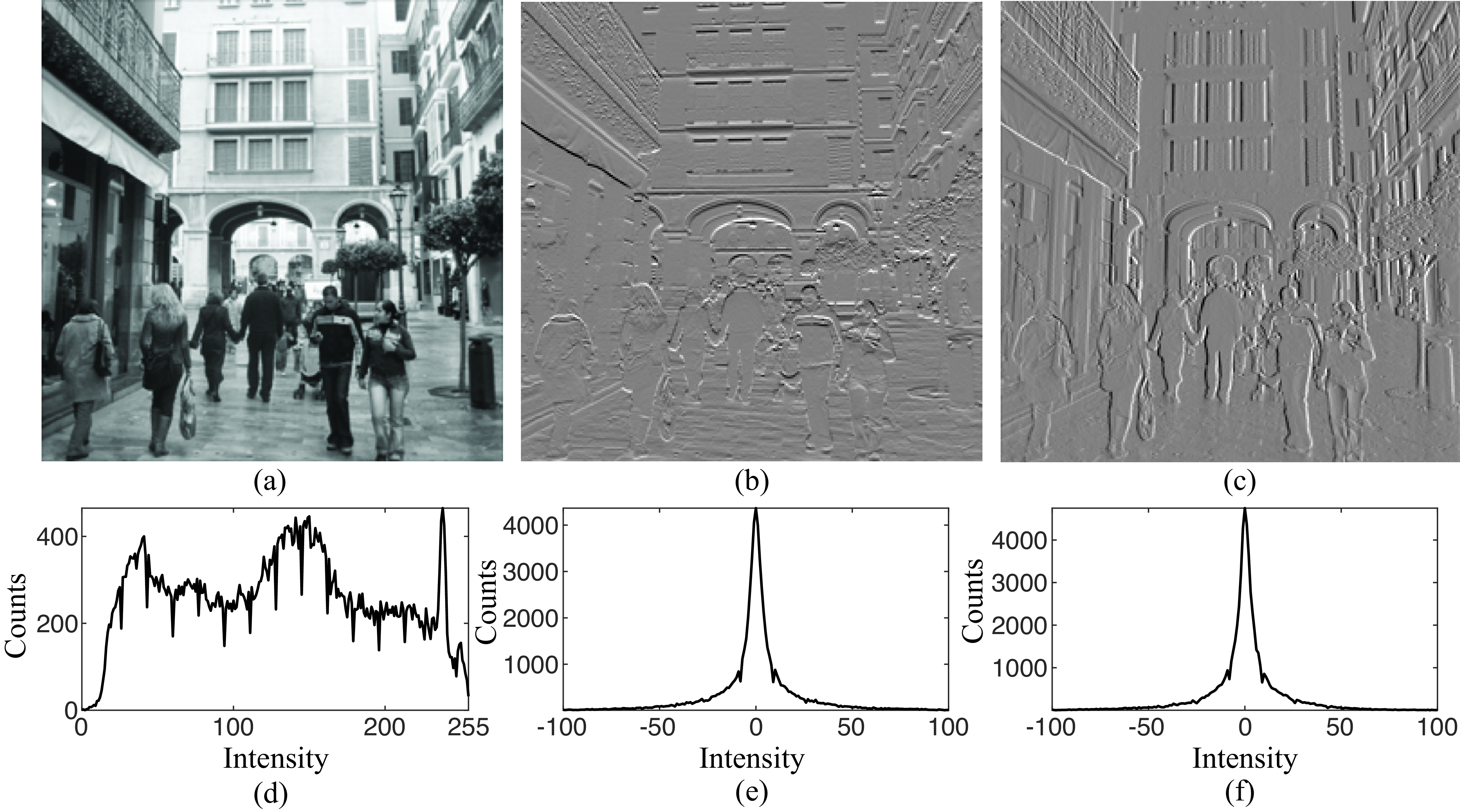
First, the histogram of an unfiltered image is already non-Gaussian. However, the image histogram does not have any interesting structure and different images have different histograms. Something very different happens to the outputs of the filters \(\left[-1,1\right]\) and \(\left[-1,1\right]^\mathsf{T}\). The histograms of the filter outputs are very clean (note that they are computed over the same number of pixels), have a unique maximum around zero, and seem to be symmetric.
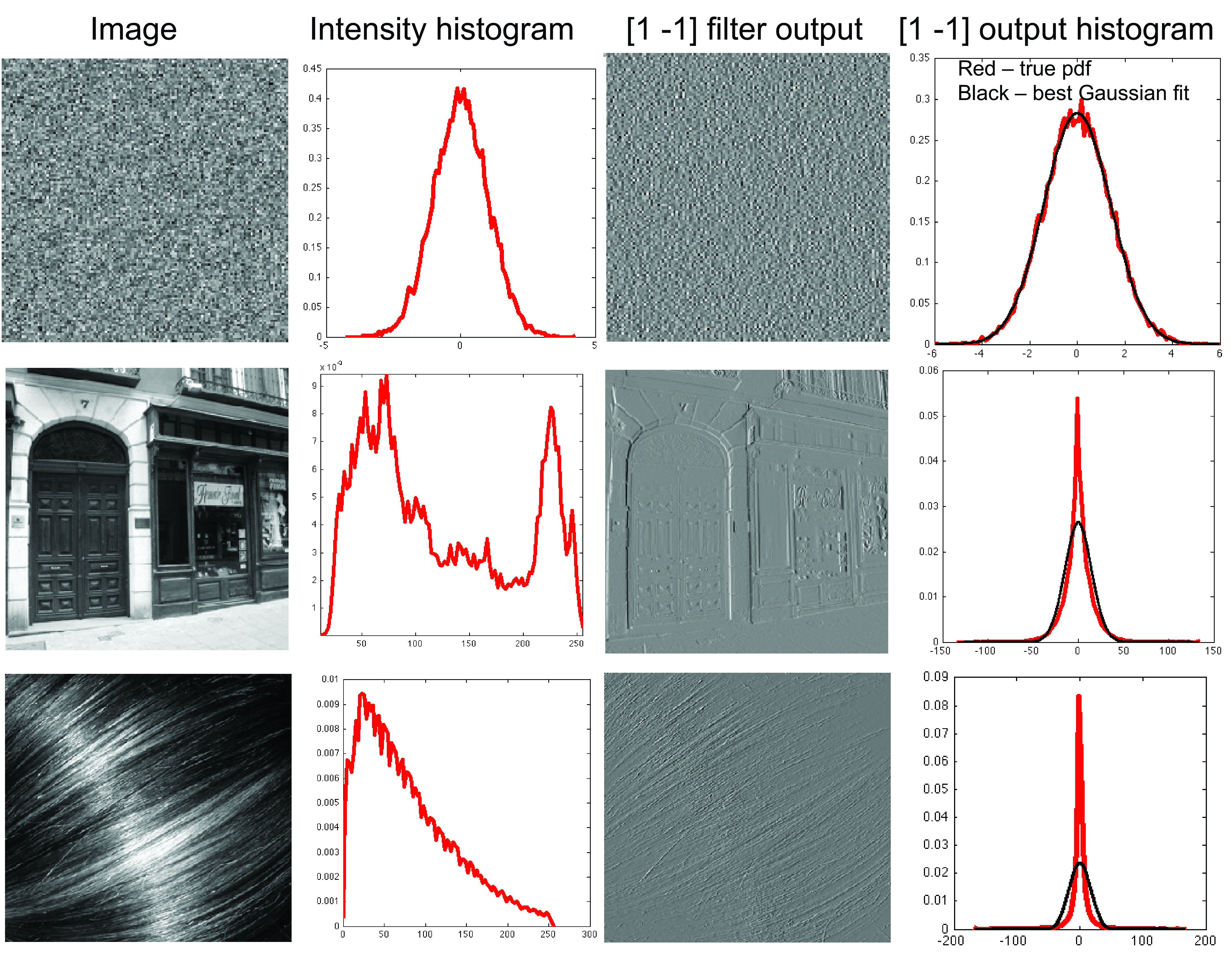
Note that this distribution of the filter outputs goes against the hypothesis of the Gaussian model. If the Gaussian image model were correct, then any filtered image would also be Gaussian, as a filtering is just a linear operation over the image. Figure 27.16 makes this point, showing histograms of band-pass filtered images (an image containing Gaussian noise, and two natural images). Note that the image subband histograms are significantly different than Gaussian.
The distribution of intensity values in the image filtered by a band-pass filter \(h\), \(\boldsymbol\ell_h = \boldsymbol\ell\circ \mathbf{h}\), can be parameterized by a simple function: \[p(\ell_h[n,m] = x) = \frac{\exp \left(- \left| x/s \right|^r \right)}{2 (s/r) \Gamma(1/r)} \tag{27.5}\]
Where \(\Gamma\) is the Gamma distribution. This function, Equation 27.5, known as the generalized Laplacian distribution, has two parameters: the exponent \(r\), which alters the distribution’s shape; and the scale parameter \(s\), which influences its variance. This distribution fits the outputs of band-pass filters of natural images remarkably well. In natural images, typical values of \(r\) lie within the range \(\left[0.4, 0.8\right]\).
Figure 27.17 shows the shape of the distribution when changing the parameter \(r\). Setting \(r=2\) gives the Gaussian distribution. With \(r=1\) we obtain the standard Laplacian distribution. When \(r \to \infty\) the distribution converges to a uniform distribution in the range \(\left[-s, s\right]\). And when \(r \to 0\), the distribution converges to a delta function.

Now that we have seen that image derivatives follow a special distribution for natural images, let’s define a statistical image model that captures the distribution of image derivatives. We can use this prior model in synthesis and noise cleaning applications.
Let’s consider a filter bank of \(K\) filters with the convolution kernels: \(h_k [n,m]\) with \(k=0, ..., K-1\). The filter bank could be composed of several Gaussian derivatives with different orientations and orders, or Gabor filters, or steerable filters from the steerable pyramid, or any other collection of band-pass filters. If we assume that the output of each filter is independent from each other (clearly, this assumption is only an approximation) we can write the following prior model for natural images: \[p(\boldsymbol\ell) = \prod_{k=0}^{K-1} \prod_{n,m} p_k(\ell_k [n,m]) \tag{27.6}\]
This distribution is the product over all filters and all locations, of how likely is each filtered value according to the distribution of natural images as modeled by the distributions \(p_k\), where \(p_k\) is a distribution with the form from equation (Equation 27.5).
To see how this model works, let’s look at a toy problem.
27.6.1 Toy Model of Image Inpainting
To build intuition about image structures that are likely under the wavelet marginal model, let’s consider a simple 1D image of length \(N=11\) that has a missing value in the middle: \[\boldsymbol\ell= \left[1,~ 1,~ 1,~ 1,~ 1,~ ?,~ 0,~ 0,~ 0,~ 0,~ 0\right]\]The middle value is missing because of image corruption or occlusion and we want to guess the most likely pixel intensity at that location. This task is called image inpainting. In order to guess the value of the missing pixel we will use the image prior models we have presented in this chapter.
We will denote the missing value with the variable \(a\). Different values of \(a\) will produce different types of steps. For instance, setting \(a=1\) or \(a=0\) will produce a sharp step edge. Setting \(a=0.5\) will produce a smooth step signal. What is the value of \(a\) that maximizes the probability of this 1D image under the wavelet marginal model?
First, we need to specify the prior distribution. For this example we will use a model specified by a single filter (\(K=1\)) with the convolution kernel \([-1, 1]\), and we will use the distribution given by equations (Equation 27.5) and (Equation 27.6). In this case, we can write the wavelet marginal model from equation (Equation 27.6) in close form. Applying the filter \(\left[-1, 1\right]\) to the 1D signal and using mirror boundary conditions, results in:
\[\boldsymbol\ell_0 = \boldsymbol\ell\circ \left[-1, 1\right] = \left[0,~0,~ 0,~0,~ 0,~ 1-a,~ a,~ 0,~ 0,~ 0,~ 0\right]\]
Now, we can use equation (Equation 27.6) to obtain the probability of \(\boldsymbol\ell\) as a function of \(a\):
\[\begin{aligned} p(\boldsymbol\ell\bigm | a) &= \prod_{n=0}^{N-1} p(\ell_0 [n] \bigm | a) = \\ %= \prod_{n} p(y [n]) \\ &= \frac {\exp \left(- \left| (1-a)/s \right|^r \right) \exp \left(- \left| a/s \right|^r \right)}{(2s/r \Gamma(1/r))^N} =\\ &= \frac{1}{(2s/r \Gamma(1/r))^N} \exp - \frac{\left| 1-a \right|^r+\left| a \right|^r} {s^r} \end{aligned} \tag{27.7}\]
Note that the first factor only depends on \(r\) and on the signal length \(N\), and the second factor depends on \(r\) and the missing value \(a\). We are interested in finding the values of \(a\) that maximize the \(p(\boldsymbol\ell\bigm | a)\) for each value of \(r\). Therefore, only the second factor is important for this analysis. Figure 27.18 plots the value of the second factor of Equation 27.7 as we vary \(a\) and \(r\). The red line represent the places where the function reaches a local maximum as a function of \(a\) for every value of \(r\).
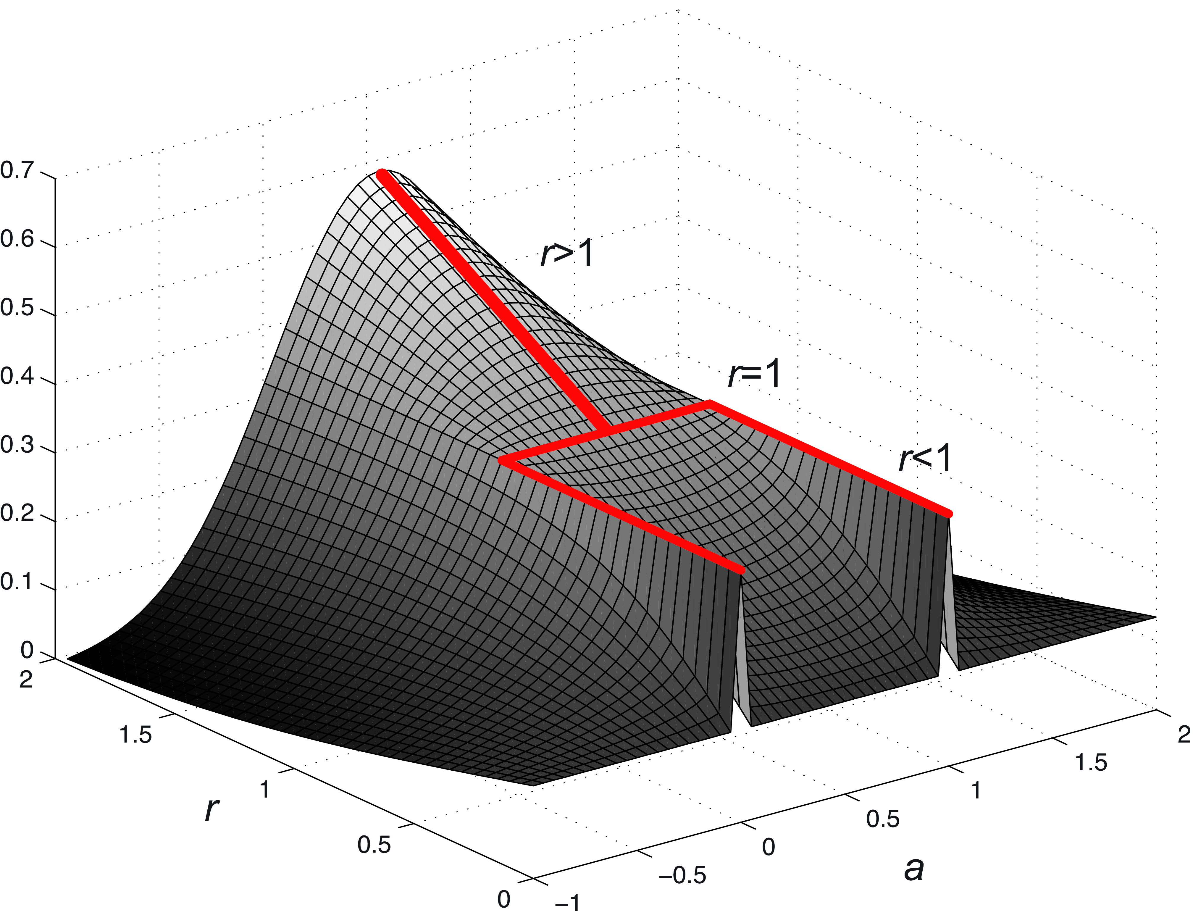
For \(r=2\) the best value of \(a\) is \(a=0.5\), and this solution is the best for any value of \(r>1\). For \(r=1\), any value \(a \in \left[0,1\right]\) is equally good, and \(p(\boldsymbol\ell)\) decreases for values of \(a\) outside that range. And for \(r<1\), the best solution is for \(a=0\) or \(a=1\). Therefore, values of \(r<1\) prefer sharp step edges. Note that \(a=0\) and \(a=1\) are both the same step edge translated by one pixel.
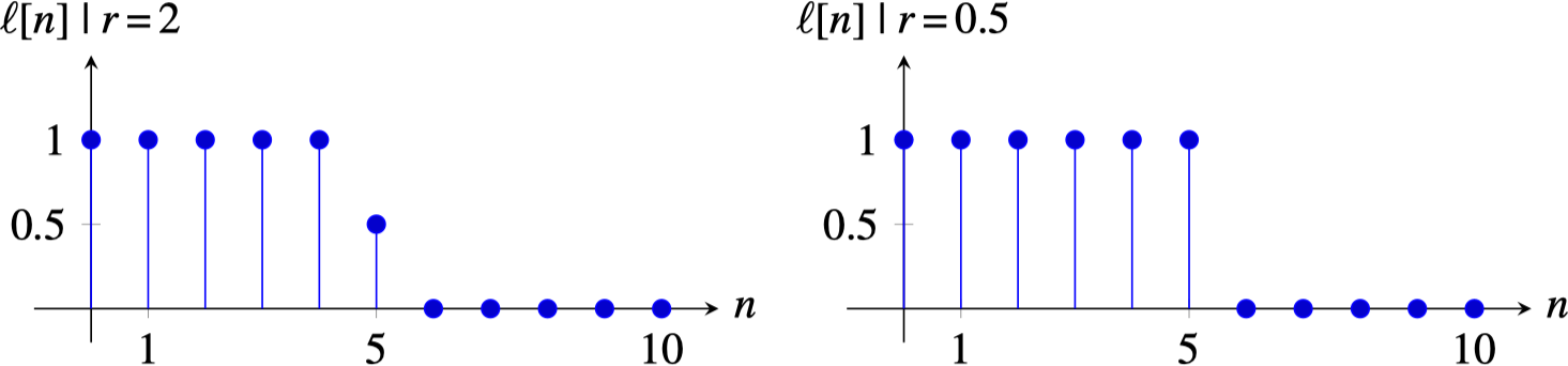
Figure 27.19 shows the final result using two different values of \(r\). When using \(r=2\), the result is a smooth signal (which is the same output we would had gotten if we had used the Gaussian image prior). The estimated value for \(a\) is the average of the nearby values. For \(r=0.5\), the result is a sharp step edge. The estimated value of \(a\) can be equal to any of the two nearby values. In the plot shown in Figure 27.19 (right) corresponds to taking the value \(a=1\).
27.6.2 Image Denoising (Bayesian Image Estimation)
The highly kurtotic distribution of band-pass filter responses in images provides a regularity that is very useful for image denoising. If we assume zero-mean additive Gaussian noise of variance \(\sigma^2\), and the observed subband coefficient value \(\hat{x} = \hat\ell_0 [n,m]\), where \(\hat\ell_0 [n,m]\) is the subband of the observed noisy input image, then the likelihood of any coefficient value, \(x=\ell_0 [n,m]\), is \[p(\hat{x} \bigm | x) \propto \exp{ \left( -\frac{(x - \hat{x})^2}{2 \sigma^2} \right) },\]where we are suppressing the normalization constants of equation (Equation 27.5) for simplicity. The prior probability of any coefficient value is the Laplacian distribution (assuming \(r=1\)) of the subbands, \[p(x) \propto \exp{ \left( -\frac{\left| x \right|}{s} \right) }.\] By Bayes rule, the posterior probability is the product of those two functions, \[P(x \bigm | \hat{x}) \propto \exp{ \left( -\frac{\left| x \right|}{s} \right)} \exp{ \left( -\frac{(x - \hat{x})^2}{2 \sigma^2} \right) } \tag{27.8}\]
The plots of Figure 27.20 show how this works. The horizontal axis for each plot is the value at a pixel of an image subband coefficient. The blue curve, showing the Laplacian prior probability for the subband values, is the same for all rows. The red line is the Gaussian likelihood and it is centered in the observed coefficient, and it is proportional to the probability that the true value had any other coefficient value. The green line shows the posterior, equation (Equation 27.8), for several different coefficient observation values. Figure 27.20 a shows the result when a zero subband coefficient is observed, resulting in the zero-mean Gaussian likelihood term (red), and the posterior (black) with a maximum at zero. In Figure 27.20 b an observation of 0.26 shifts the likelihood term, but the posterior still has a peak at zero. And in Figure 27.20 c an observed coefficient value of 1.22 yields a maximum posterior probability estimate of 0.9.
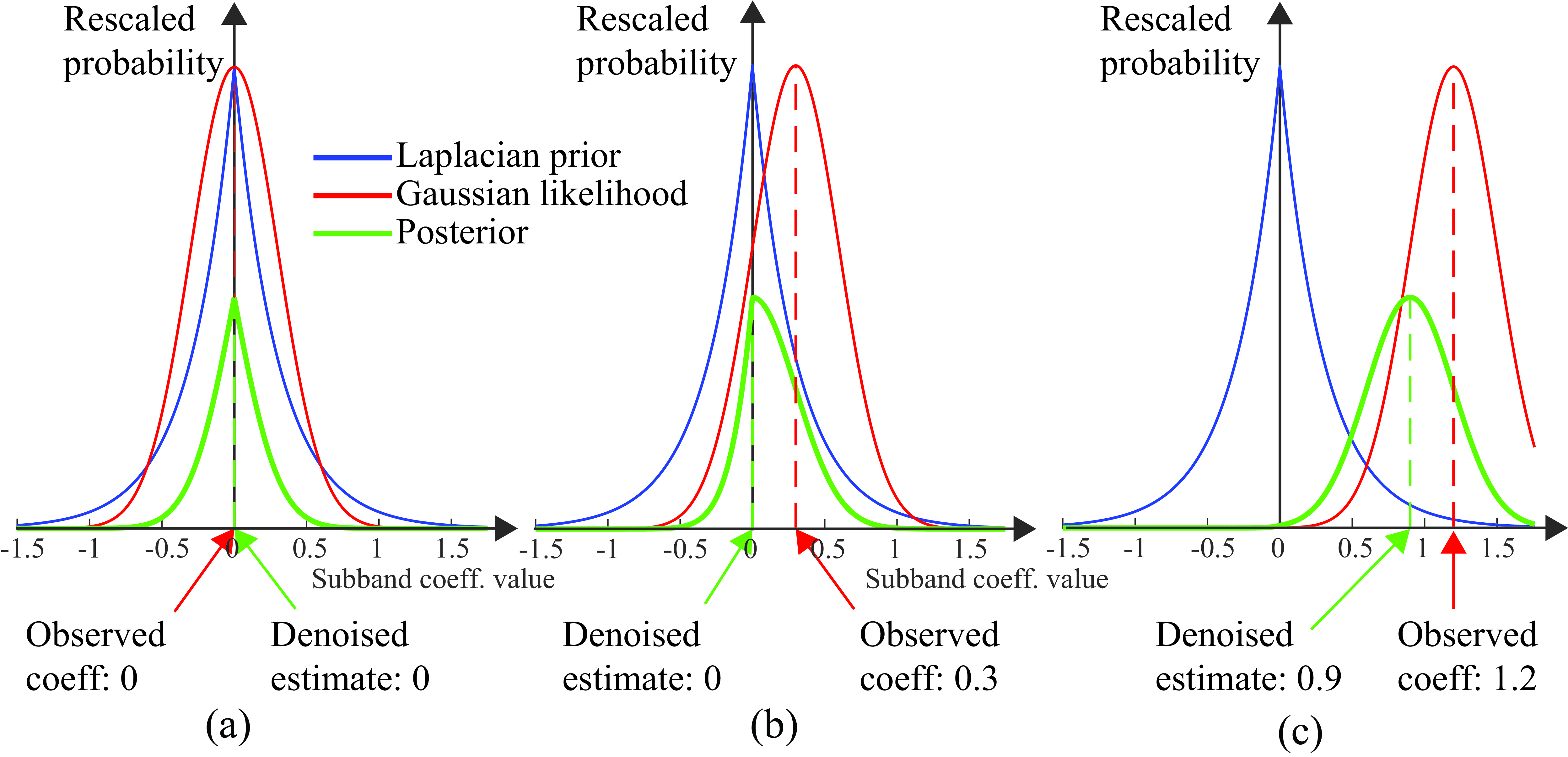
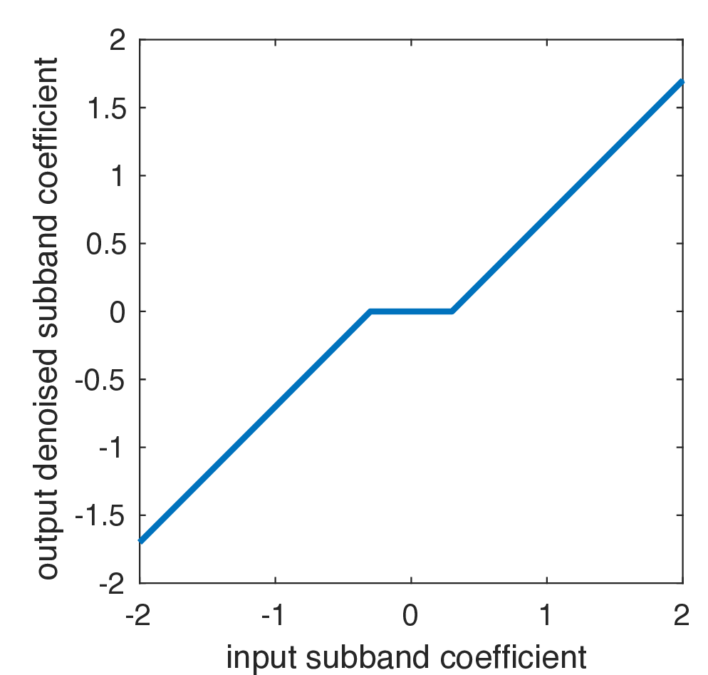
Figure 27.21 shows the resulting look-up table to modify the noisy observation to the MAP estimate for the denoised coefficient value. Note that this implements a coring function [12]: if a coefficient value is observed near zero, it is set to zero, based on the very high prior probability of zero coefficient values.
For a more detailed analysis and examples of denoising using the Laplacian image prior, we refer the reader to the work of Eero Simoncelli [12].
27.7 Nonparametric Markov Random Field Image Models
The Gaussian and kurtotic wavelet image priors both involve modeling the image as a sum of statistically independent basis functions, Fourier basis functions, in the case of the Gaussian model, or wavelets, in the case of the wavelet image prior.
A powerful class of image models is known as Markov random field (MRF) models. They have a precise mathematical form, which we will describe later, in Chapter 29. For now, we present the intuition for these models: if the values of enough pixels surrounding a given pixel are specified, then the probability distribution of the given pixel is independent of the other pixels in the image. To fit and sample from the MRF structure requires the mathematical tools of graphical models, to be introduced in Chapter 29. As we will see in the following chapter, Efros and Leung [13] introduced an algorithm for texture synthesis that exploits intuitions about the Markov structure of images to synthesize textures that are visually compelling. The intuition of the Efros and Leung texture generation model is that if you condition on a large enough region of nearby pixels around a center pixel, that effectively determines the value of the central pixel. We will study this algorithm in more detail in the next chapter devoted to texture analysis and synthesis Chapter 28. We will focus here on a similar algorithm for the problem of image denoising.
27.7.1 Denoising Model (Nonlocal Means)
Baudes, Coll, and Morel made use of that intuition to define the nonlocal means denoising algorithm [14]. The nonlocal means denoised image is a weighted sum of all other pixels in the image, weighted by the similarity of the local neighborhoods of each pair of pixels. More formally, \[\ell_{\mbox{NLM}}[n,m] = \sum_{k,l} w_{n,m}[k,l] \ell[k,l]\] where \[w_{n,m}[k,l] = \frac{1}{Z_{n,m}} \exp{\frac{- \left| \ell[N_{k,l}] - \ell[N_{n,m}] \right| ^2}{h^2}}, \tag{27.9}\] where \(N_{i, j}\) denotes an \(h \times h\) region of pixels centered at \(i, j\), and \(Z_{n,m}\) is set so that the weights over the image sum to one, that is \(\sum_{kl} w_{n,m}[k,l] = 1\).
Figure 27.22 shows the weighting functions for two images. The parameter \(h\) is typically set to \(10 \sigma\), where \(\sigma\) is the estimated image noise standard deviation. Within Figure 27.22 (a and b) at left is a grayscale image where the center position of interest to be denoised is marked with a white star. The right side of the figures shows for some value of \(h\) in equation Equation 27.9 the weighting function \(w_{n,m}[k,l]\) indicating which pixels are averaged together to yield the nonlocal mean value placed at the starred location in the denoised image. Note, for both Figure 27.22 (a and b) the sampling at image regions with similar local structure as the image position to be denoised.
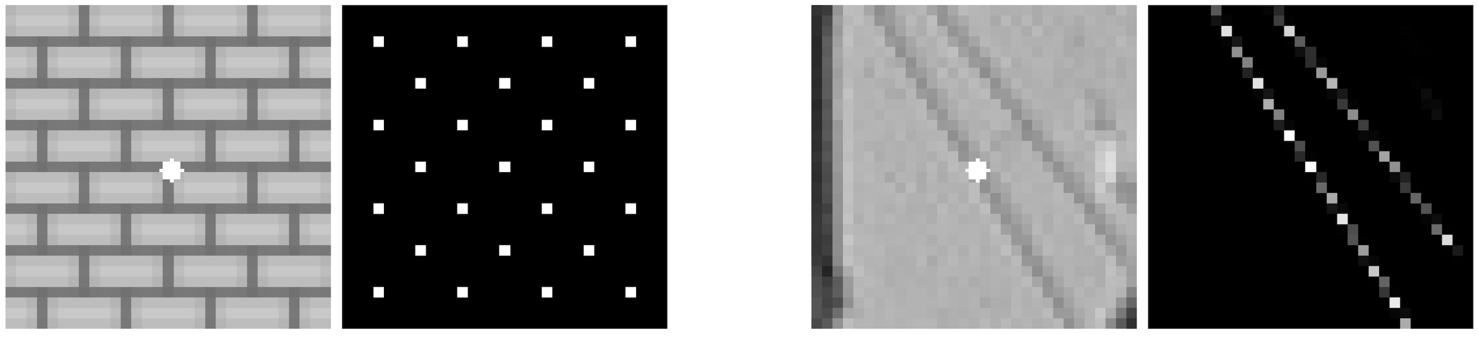
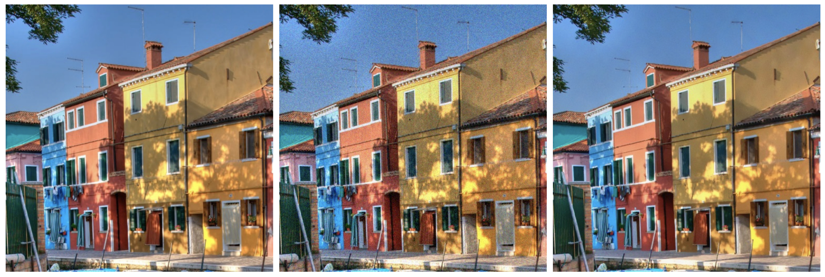
Figure 27.23 shows the result on a real image. On the left is the original image. The middle image is with additive Gaussian noise added, that is, \(\sigma=15\) for 0–255 image scale. On the right is the result, showing the image with nonlocal means noise removed.
27.8 Concluding Remarks
The models presented in this chapter do not try to understand the content of the pictures, but utilize low-level regularities of images in order to build a statistical model. Modeling these statistical regularities enable many tasks, including both image synthesis and image denoising.
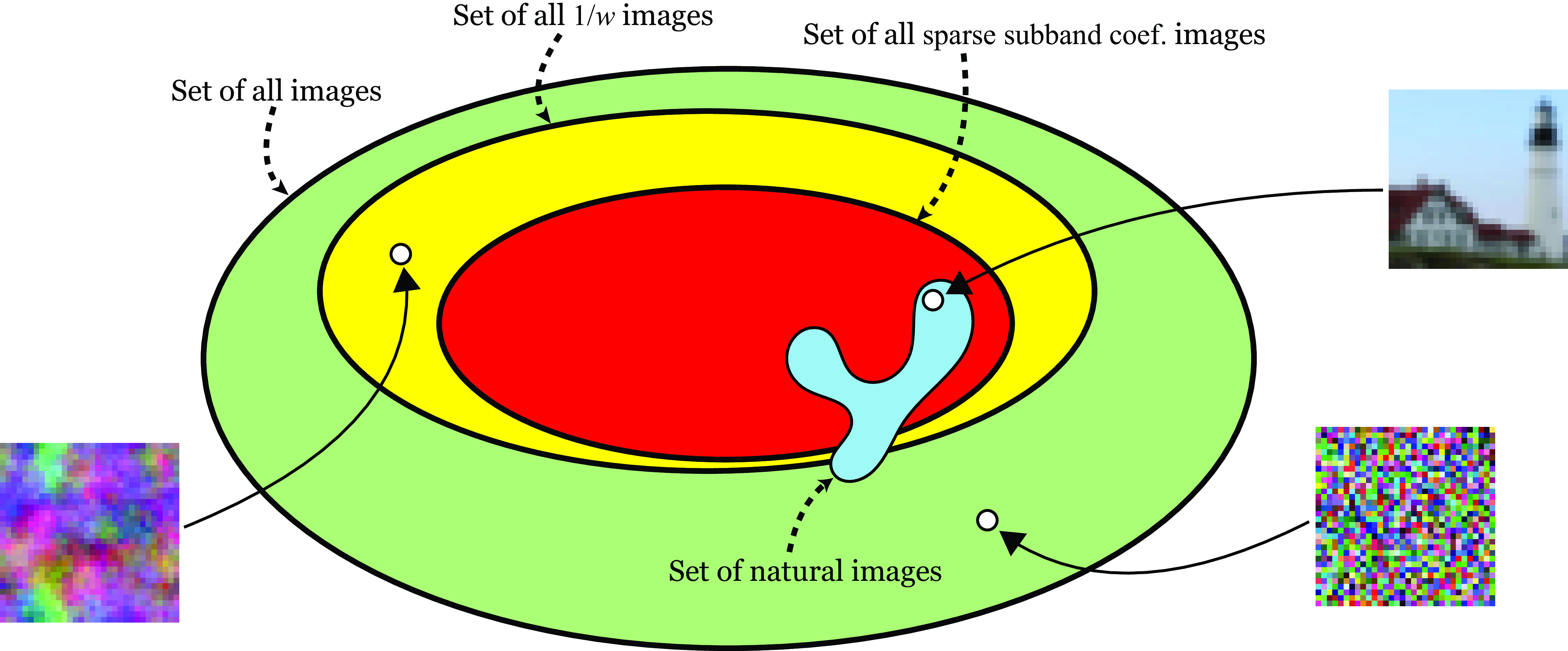
We have seen some simple models that try to constrain the space of natural images. These models, despite their simplicity, are useful in several applications. However, they fail in providing a strong image model that can be used to sample new images. As illustrated in Figure 27.24 the sequence of models we have studied in this chapter, only help in reducing a bit the space of possible images.
We will see stronger generative image models in Chapter 32.