8 Color
8.1 Introduction
There are many benefits to sensing color. Color differences let us check whether fruit is ripe, tell whether a child is sick by looking at small changes in the color of the skin, and find objects in clutter.
We’ll begin our study of color by describing the physical properties of light that lead to the perception of different colors. Then we’ll describe how humans and machines sense colors, and how to build a system to match the colors perceived by an observer. We’ll briefly describe how to represent color–different color coordinate systems. Finally, we’ll describe how spatial resolution and color interact.
8.2 Color Physics
Isaac Newton revealed several intrinsic properties of light in experiments summarized by his drawing in Figure 8.1. A pinhole of sunlight enters through the window shade, and a lens focuses the light onto a prism. The prism then divides the white light into many different colors. These colors are elemental: if one of the component colors is passed through a second prism, it doesn’t split into further components.
Newton understood that white light could be decomposed into different colors and invented the term spectrum.
Our understanding of light and color explains such experiments. Light is a mixture of electromagnetic waves of different wavelengths. Sunlight has a broad distribution of light of the visible wavelengths. At an air/glass interface, light bends in a wavelength-dependent manner, so a prism disperses the different wavelength components of sunlight into different angles, and we see different wavelengths of light as different colors. Our eyes are sensitive to only the narrow band of that electromagnetic spectrum, the visible light, from approximately 400 nm to 700 nm, which appears blue to deep red, respectively.
The bending of light at a material boundary is called refraction, and its wavelength dependence lets the prism separate white light into its component colors. A second way to separate light into its spectral components is through diffraction, where constructive interference of scattered light occurs in different directions for different wavelengths of light.
Figure 8.2 (a) shows a simple spectrograph, an apparatus to reveal the spectrum of light, based on diffraction from a compact disk (CD) [2]. Light passes through the slit at the right, and strikes a CD (with a track pitch of about 1,600 nm). Constructive interference from the light waves striking the CD tracks will occur at a different angle for each wavelength of the light, yielding a separation of the different wavelengths of light according to their angle of diffraction. The diffracted light can be viewed, Figure 8.2 (b), or photographed through the hole at the bottom left of the photograph. The spectrograph gives an immediate visual representation of the spectral components of colors in the world. Some examples are shown in Figure 8.3.
8.2.1 Light Power Spectra
The light intensity at each wavelength is called the power spectrum of the light. The color appearance of light is determined by many factors, including the image context in which the light is viewed; but a very important factor in determining color appearance is the power spectrum. In this initial discussion of color, we will assume that the power spectrum of light determines its appearance, although you should remember that this is true only within a fixed visual context.
Why does the sky look blue? And why does it look orange during a sunset? 
Figure 8.3 shows a spectrograph visualization of some light power spectra (the right image of each row) along with the image that the spectrograph was pointed toward (left images). Figure 8.4 shows the spectrum of a blue sky, plotted as intensity as a function of wavelength.


8.2.2 The Color Appearance of Different Spectral Bands
It is helpful to develop a feel for the approximate color appearance of different light spectra. Again, we say the approximate appearance because the subjective appearance can change according to other factors than just the spectrum.
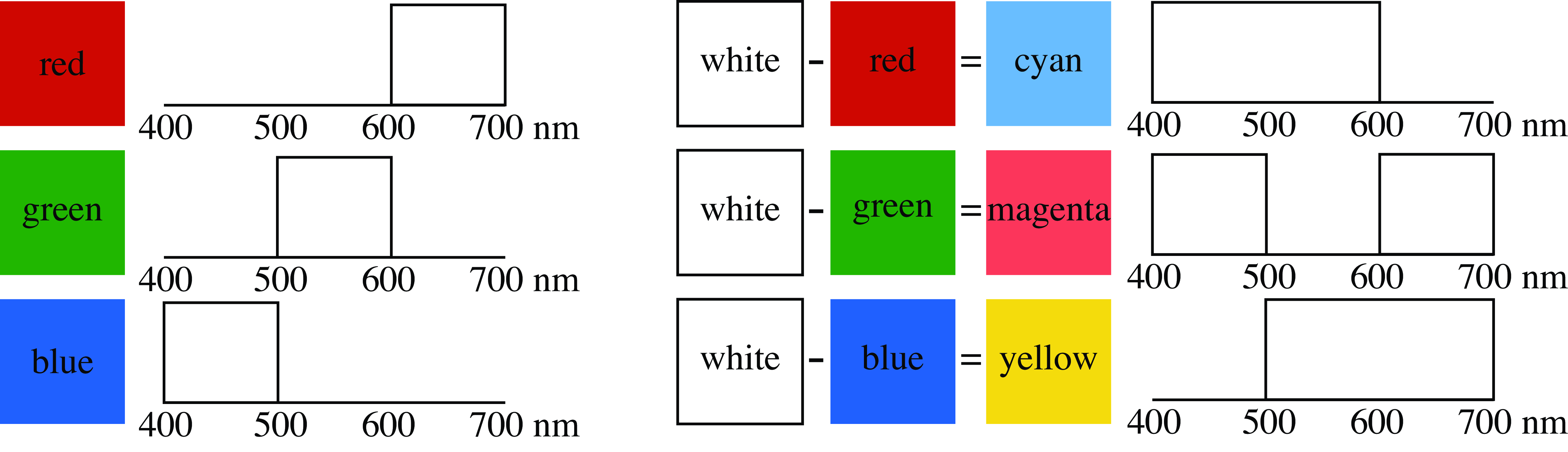
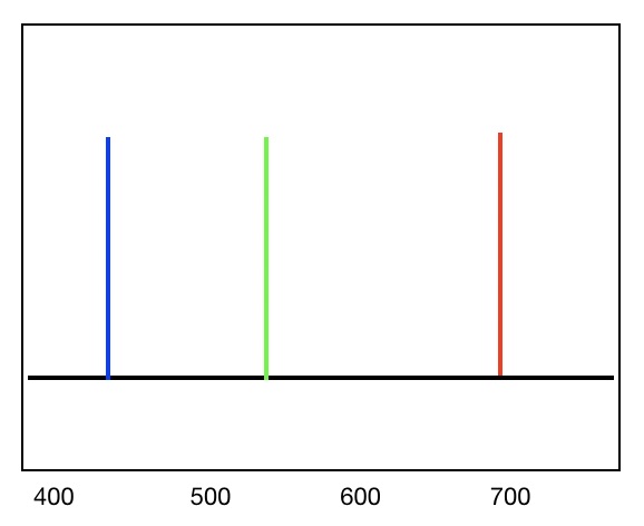
The visible spectrum lies roughly in the range between 400 and 700 nm, see Figure 8.5. We can divide the visible spectrum into three 100 nm bands, and study the appearance of light power spectra where power is present or absent from each of those three bands, in all of the eight (\(2^3\)) possible combinations.
Light with spectral power distributed in just the 400–500 nm wavelength band will look some shade of blue, the exact hue depending on the precise distribution. Light in the 500–600 nm band will appear greenish. Most distributions within the 600–700 nm band will look red.
White light is a mixture of all spectral colors. A spectrum of light containing power evenly distributed over 400—700 nm would appear approximately white. Light with no power in any of those three bands, that is, darkness, appears black.
There are three other spectral classes left in this simplified grouping of spectra: spectral power present in two of the spectral bands, but missing in the third. Cyan is a combination of both blue and green, or roughly spectral power between 400 and 600 nm. In printing and color film applications, this is sometimes called minus red, since it is the spectrum of white light, minus the spectrum of red light. The blue and red color blocks, or light in the 400–500 nm band, and in the 600–700nm band, is called magenta, or minus green. Red and green together, with spectral power from 500–700 nm, make yellow, or minus blue Figure 8.6.
8.2.3 Light Reflecting from Surfaces
When light reflects off a surface, the power spectrum alters in ways that depend on the surface’s characteristics and geometry. These changes in light allow us to perceive objects and surfaces by observing their influence on the reflected light.
The interaction between light and a surface can be quite complex. Reflections can be specular or diffuse, and the reflected power spectrum may depend on the relative orientations of the incident light, surface, and the observed reflected ray. In its full generality, the reflection of light from a surface is described by the bidirectional reflectance distribution function (BRDF) [4], [5]. For this discussion, we will focus on diffuse surface reflections, where the power spectrum of the reflected light, \(r(\lambda)\), is proportional to the wavelength-by-wavelength product of the power spectrum of the incident light, \(\ell_{\texttt{in}}(\lambda)\), and a reflectance spectrum, \(s(\lambda)\), of the surface: \[r(\lambda) = k \ell_{\texttt{in}}(\lambda) s(\lambda),\]
where the proportionality constant \(k\) depends on the reflection geometry. This diffuse reflection model characterizes most matte reflections. Such wavelength-by-wavelength scaling is also a good model for the spectral changes to light caused by transmission through an attenuating filter. The incident power spectrum is then multiplied at each wavelength by the transmittance spectrum of the attenuating filter.
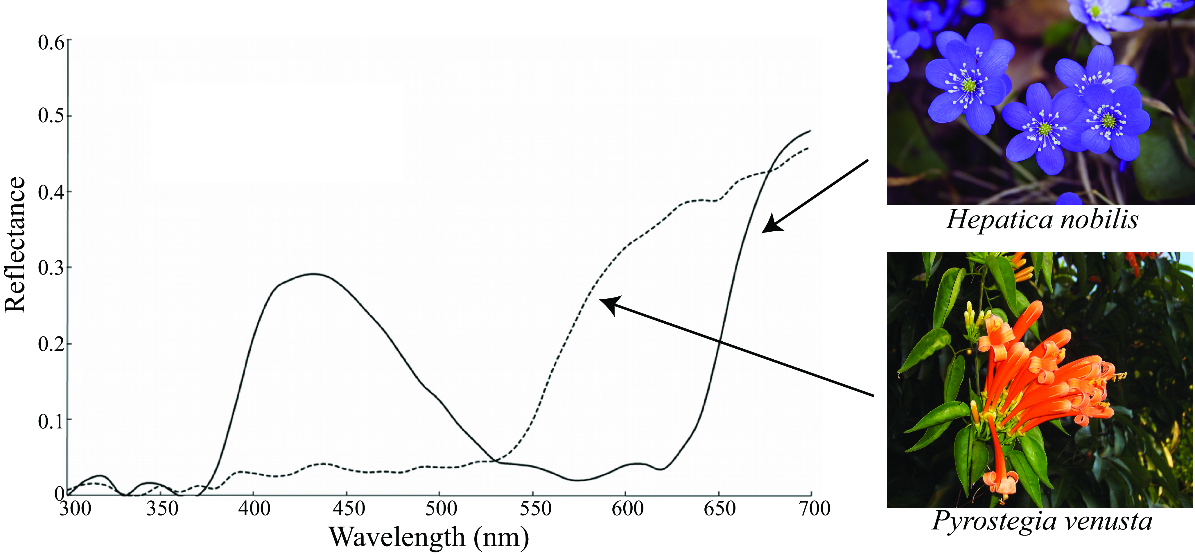
Some reflectance spectra of real-world surfaces are plotted in Figure 8.7. The flower Hepatica Nobilis (solid line) is blue, while Pyrostegia venusta (dotted line) is orange.
The reflectance spectrum of a surface often carries valuable information about the material being viewed, such as whether a fruit is ripe, whether a human’s skin is healthy, or whether the material differs from another viewed material. It may be the case that a low-dimensional version of the surface reflectance spectrum is sufficient for many visual tasks, and as we see subsequently, the human visual system represents color with only three numbers. So it is an important visual task to estimate either the surface reflectance spectrum, or a low-dimensional summary of it.
To estimate surface colors by looking, a vision system has the task of estimating the illumination spectrum and the surface reflectance spectra, from observations of only their products. When the illumination is white light with equal power in all spectral bands, the observed reflected spectrum is proportional to the reflectance spectrum of the material itself. However, under the more general condition of unknown illumination color, a visual system will need to estimate the surface reflectance spectrum, or projections of it, by taking the context of nearby image information into account.
There are many proposed algorithms to do that, ranging from heuristics, for example, assuming the color of the brightest observed object is white [9], to statistical methods [10] and neural network based approaches [11]. Even humans don’t solve the problem perfectly or consistently, revealed especially through the internet meme of #TheDress [12], shown in Figure 8.8.
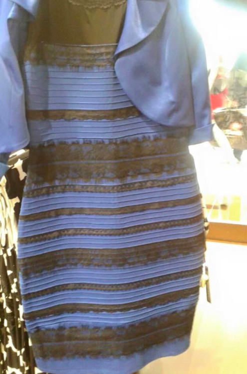
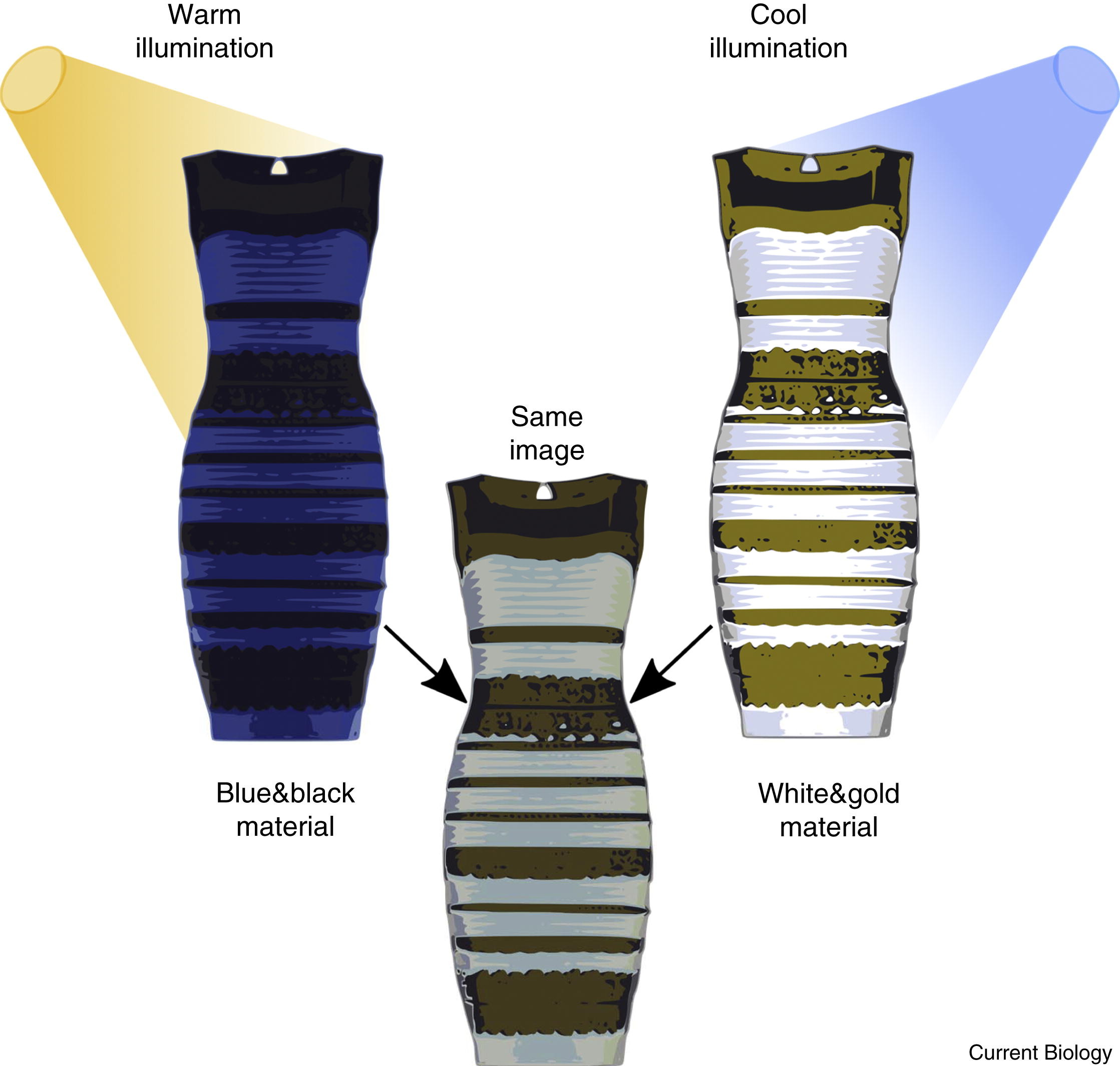
The perceived colors of the dress depend on the assumed color of the illumination, and people can disagree significantly about the colors they see [13]. The assumption of a warm, yellowish, illumination color leads to a perception of blue and black material. The assumption of a cool, blueish illumination leads to a perception of white and gold material. Both perceptions are consistent with the observed product of illumination and reflectance seen in the dress image.
Did you perceive the dress, Figure 8.8, to be black on blue, or gold on white? Can you make the perception change?
While such context-dependent effects are important in color perception, as we quantify color perception we will assume that our perception of color depends only on the spectrum of light entering the eye. This will serve us well for many industrial applications.
8.3 Color Perception
Now we turn to our perception of color. We first describe the machinery of the eye, then describe some methods to measure color appearance. These methods to measure color appearance implicitly assume a white illumination spectrum, but they often serve the needs of industry and science.
8.3.1 The Machinery of the Eye
An instrument such as a spectrograph (Figure 8.2 shows a simple one) can measure the light power spectrum at hundreds of different wavelengths within the visible band, yielding hundreds of numbers to describe the light power spectrum. Despite this, a useful description of the visual world can be obtained from a much lower dimensional description of the light power spectrum.
The retina contains photoreceptors called the rod and cones. Rods are used in low-light levels, and the cones are used in color vision. In low-light, only the rods operate and our vision becomes black and white.
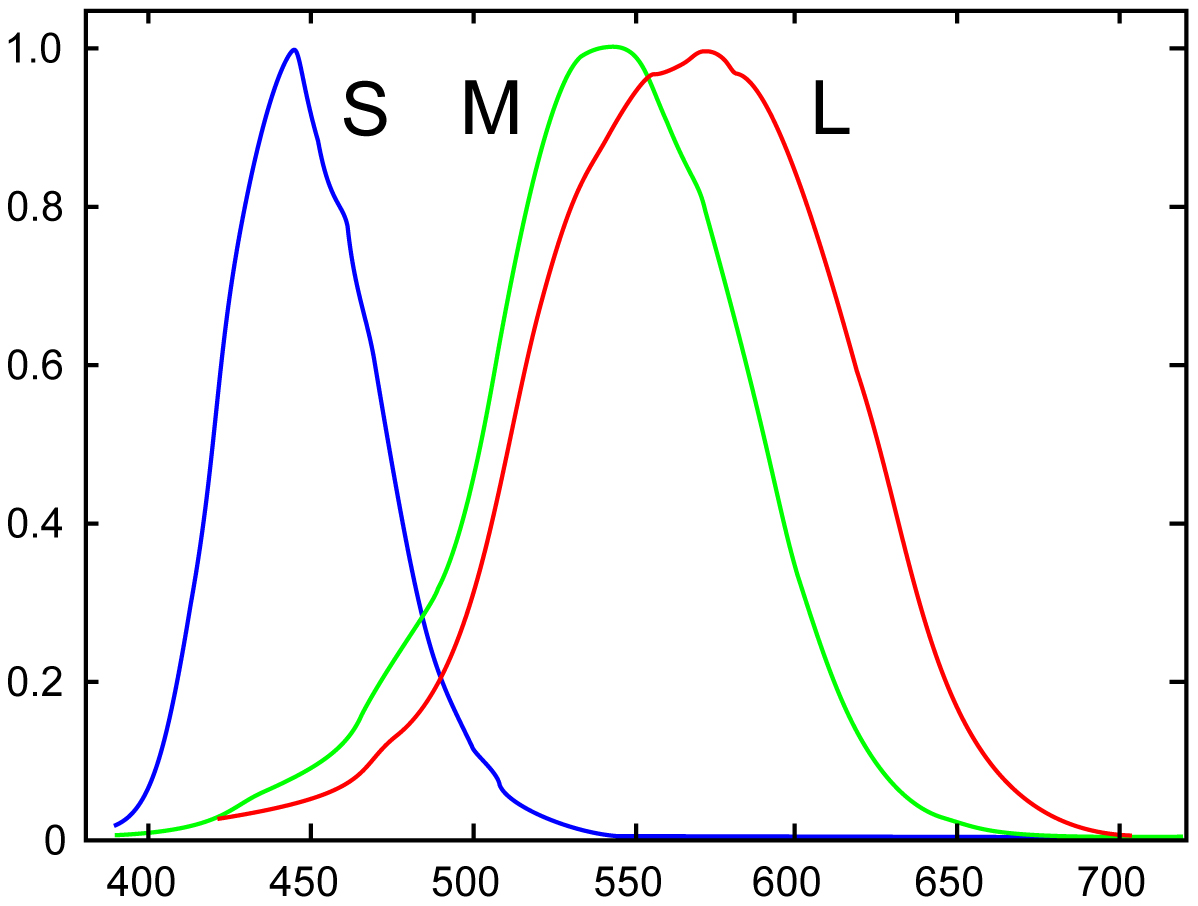
The human visual system analyzes the incident light power spectrum with only three different classes photoreceptors, called the L, M, and S cones because they sample at the long, medium, and short wavelengths. This gives the human visual system a three-dimensional (3D) description of light, with each photoreceptor class taking a different weighted average of the incident light power spectrum.
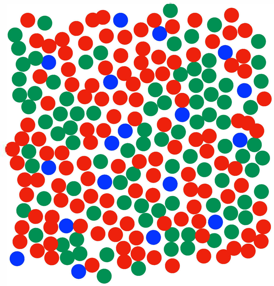
Figure 8.9 (a) shows the spatial sampling pattern, for each of the three cone classes, measured from a subject’s eye [14]. The L cones are colored red, the M cones green, and the S cones are colored blue. Note the hexagonal packing of the cones in the retina, and the stochastic assignment of L, M, and S cones over space. Note also the much sparser spatial sampling of the S cones than of either the L or M cones. Figure 8.9 (b) shows the spectral sensitivity curves for the L, M, and S cones. This sampling pattern was measured from near the fovea, where there are no rods, and the cones are close-packed.
We can describe the photoreceptor responses using matrix algebra. If the matrix \(\mathbf{C}_{\mbox{eye}}\) consists of the spectral sensitivities of the L, M, and S cones in three rows, and the vector \(\mathbf{t}\) is a column vector of the spectrum of light incident on the eye, then the L, M, and S cone responses will be the product, \[\begin{bmatrix} L \\ M \\ S \\ \end{bmatrix} = \mathbf{C}_{\mbox{eye}} \, \mathbf{t} \tag{8.1}\]
The fact that our eyes have three different classes of photoreceptors has many consequences for color science. It determines that there are three primary colors, three color layers in photographic film, and three colors of dots needed to render color on a display screen. In the next section, we describe how to build a color reproduction system that matches the colors seen in the world by a human observer.
8.3.2 Color Matching
Color science tells us how to analyze and reproduce color. We seek to build image displays so that the output colors match those of some desired target, and to manufacture items with the same colors over time. Much of the color industry revolves around the ability to repeatably control colors. Colors can be trademarked (Kodak Yellow, IBM Blue) and we have color standards for foods. Figure 8.10 shows French fry color standards.

One of the tasks of color science is to predict when a person will perceive that two colors match. For example, we want to know how to adjust a display to match the color reflecting off some colored surface. Even though the spectra may be very different, the colors can almost always be made to match.
It is possible to infer human color matching performance by examining the spectral sensitivity curves of the receptors shown in Figure 8.9 (b). We attempt to match a color using a combination of reference colors, typically called primary colors. Through experimentation, it has been discovered that the appearance of any color can be matched through a linear combination of three primary colors. This is due to the presence of three classes of photoreceptors in our eyes. It has also been found that these color matches are transitive—if color A matches a particular combination of primaries and color B matches the same combination of primaries, then color A will match color B. Consequently, the amount of each primary required to match a color can serve as a set of coordinates indicating color [17].
8.3.3 Color Metamerism
Two different spectra are metameric if they appear to be the same color to our eyes. There is a large space of metamers: any two vectors describing light power spectra that give the same projection onto a set of color matching functions will look the same to our eyes. There’s a high-dimensional space of light spectra, and we’re only viewing projections onto a 3D subspace in the colors we see.
Do spotlights on produce in a supermarket help good and bad fruit become metameric matches?
In practice, the three projections we observe capture much of the interesting action in images. Hyperspectral images (recorded at many different wavelengths of analysis) add some, but not a lot, to the image formed by our eyes.
8.3.4 Linear Algebraic Interpretation of Color Matching
In this chapter, we assume that color appearance is determined by the light spectrum reaching the eye. In reality, numerous factors can influence color appearance, including the eye’s state of brightness adaptation, ambient illumination, and surrounding colors. However, a color matching system that relies solely on the light spectrum will still perform well.
To measure the color associated with a light spectrum \(\mathbf{t}\) we need to be able to predict the eye’s responses to the spectrum. From equation (Equation 8.1), the task of color measurement is to find the projection of a given light spectrum into the special 3D subspace defined by the eye’s cone spectral response curves. Any basis for that 3D subspace will serve that task, so the three basis functions do not need to be the color sensitivity curves of Figure 8.9 themselves. They can be any linear combination of them, as well.
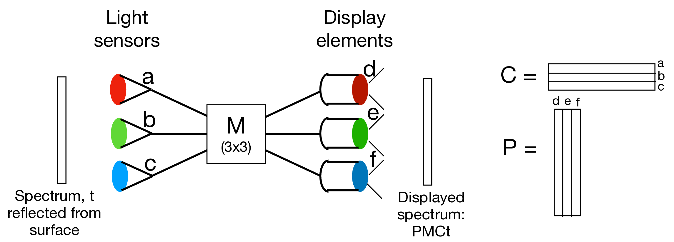
We can define a color reproduction system, Figure 8.11, by first specifying its three spectral sensitivity curves. We put these into the \(3 \times N\) matrix, \(\mathbf{C}\), where \(N\) is the number of spectral samples over the visible illumination range. As discussed previously, the three curves, \(\mathbf{C}\), should be a linear combination of the eye’s spectral sensitivity curves, or \[ \mathbf{C} = \mathbf{R} \, \mathbf{C}_{\mbox{eye}}, \tag{8.2}\] where \(\mathbf{R}\) is any full-rank \(3 \times 3\) matrix. We can translate between any two different color spaces by applying a general \(3 \times 3\) matrix transformation to change basis vectors. Note, the basis vectors do not need to be orthogonal, and most color system basis vectors are not.
8.3.5 Color Matching Functions and Primary Lights
A color reproduction system measures an input light and produces an output light that matches the color appearance of the input light. A camera with a screen display is an example of a color reproduction system, as the colors of objects in the world are measured, then reproduced on the screen display of the camera. We can match the eye’s response to a given light spectrum through the appropriate control of a sum of three lights, which we’ll call the primary lights. For the example of a display screen, the three color elements of each pixel are the primary lights.
Because the eye’s photosensors respond in linear proportion to the amount of the incoming light spectrum within its spectral sensitivity curve, the rules of linear algebra apply to color manipulation. For a given set of three primary lights, the strengths of each primary light can be adjusted to obtain a visual match to a desired color. There is one exception to this: because primary lights can only be combined in positive values, some input colors are outside the gamut—the range of colors that can be produced—of a the positive combination of a given set of primary lights.
The color reproduction system is then defined by two sets of spectral curves and a \(3 \times 3\) matrix, \(\mathbf{M}\), see Figure 8.11. The first set are the spectral sensitivities as a function of wavelength for each of the three photosensors. We write each of those spectral curves as a row vector of a matrix, \(\mathbf{C}\). The \(3 \times 3\) matrix, \(\mathbf{M}\), translates any color measurement to a set of amplitude controls for the primary lights, \(\mathbf{P}\). The second set of spectral curves of a color reproduction system are the spectra of the three primary lights, which we write as column vectors of the matrix, \(\mathbf{P}\).
For a given set of primary lights, \(\mathbf{P}\), we seek to find a matrix of color sensitivity curves, \(\mathbf{C}\), and \(3 \times 3\) matrix, \(\mathbf{M}\), which allow perfect reproduction of colors, as viewed by a human observer. Here, we derive the conditions that \(\mathbf{P}\), \(\mathbf{C}\), and \(\mathbf{M}\) must satisfy to allow for perfect reproduction of colors.
Let the spectrum of the light reflecting from the surface to be matched in color be \(\mathbf{t}\). The eye’s response to that light is modeled as the sum of a term-by-term multiplication of the spectral sensitivities of each photoreceptor, in the rows of \(\mathbf{C}_{\mbox{eye}}\) times the spectrum of the light. Thus, the responses of the eye to that spectrum will be the \(3 \times 1\) column vector, \(\mathbf{C}_{\mbox{eye}} \mathbf{t}\).
We can write the response of the eye to the output of the color matching system as the following matrix products. The light impinging on the sensors (a, b, c in Figure 8.11) of the color matching system will give responses \(\mathbf{C} \mathbf{t}\) and controls \(\mathbf{M} \mathbf{C} \mathbf{t}\) to the primary lights. If this output modulates the corresponding primary lights (d, e, and f in Figure 8.11), then the light displayed by the color matching system will be \(\mathbf{P} \mathbf{M} \mathbf{C} \mathbf{t}\). We want this spectrum to give the same responses in the eye as the original reflected color, thus we must have: \(\mathbf{C}_{eye} \mathbf{P} \mathbf{M} \mathbf{C} \mathbf{t} = \mathbf{C}_{eye} \mathbf{t}\). Because that relation must hold for any input vector \(\mathbf{t}\), we must have \[ \mathbf{C}_{eye} \mathbf{P} \mathbf{M} \mathbf{C} = \mathbf{C}_{eye} \tag{8.3}\]
What conditions on \(\mathbf{P}\) and \(\mathbf{C}\) are required for equation (Equation 8.3) to hold? First, the subspace of the eye responses \(\mathbf{C}_{eye}\) must be the same as that measured by the color sensing system, \(\mathbf{C}\). If that weren’t the case, then perceptibly different spectra could map onto the same color sensing system measurements. So we must have \(\mathbf{C} = \mathbf{R} \mathbf{C}_{eye}\), for some full-rank \(3 \times 3\) matrix, \(\mathbf{R}\) (with inverse \(\mathbf{R}^{-1}\)). Substituting this twice into equation (Equation 8.3) gives \[ \mathbf{R}^{-1} \mathbf{C} \mathbf{P} \mathbf{M} \mathbf{R} \mathbf{C}_{eye} = \mathbf{C}_{eye} \tag{8.4}\]
From Equation 8.4 it follows that \(\mathbf{C} \mathbf{P} \mathbf{M} = \mathbf{I}_3\), the \(3 \times 3\) identity matrix. These conditions on the spectral sensitivities, \(\mathbf{C}\), the display spectra, \(\mathbf{P}\) and the sensors-to-primaries mixing matrix, \(\mathbf{M}\) for a color reproduction system are summarized below:
\[\begin{aligned} \mathbf{C} &= \mathbf{R} \mathbf{C}_{\mbox{eye}} \end{aligned} \tag{8.5}\]
\[\begin{aligned} \mathbf{M} &= (\mathbf{C P})^{-1}, \end{aligned} \tag{8.6}\]
where \(\mathbf{C}_{\mbox{eye}}\) are the human photoreceptor sensitivities and \(\mathbf{R}\) is a full-rank \(3 \times 3\) matrix.
Conditions required for color matching in the color reproduction system of Figure 8.11.
Figure 8.12 displays the elements of two matrices \(\mathbf{C}\) and \(\mathbf{P}\) that define a valid color matching system. For a color reproduction system to be physically realizable, the elements of the primary spectra, \(\mathbf{P}\), must be non-negative.
Because many color sensitivity matrices \(\mathbf{C}\) can satisfy Equation 8.5 some standardized color sensitivity matrices have been adopted to allow common representations of colors.
8.3.6 CIE Color Space
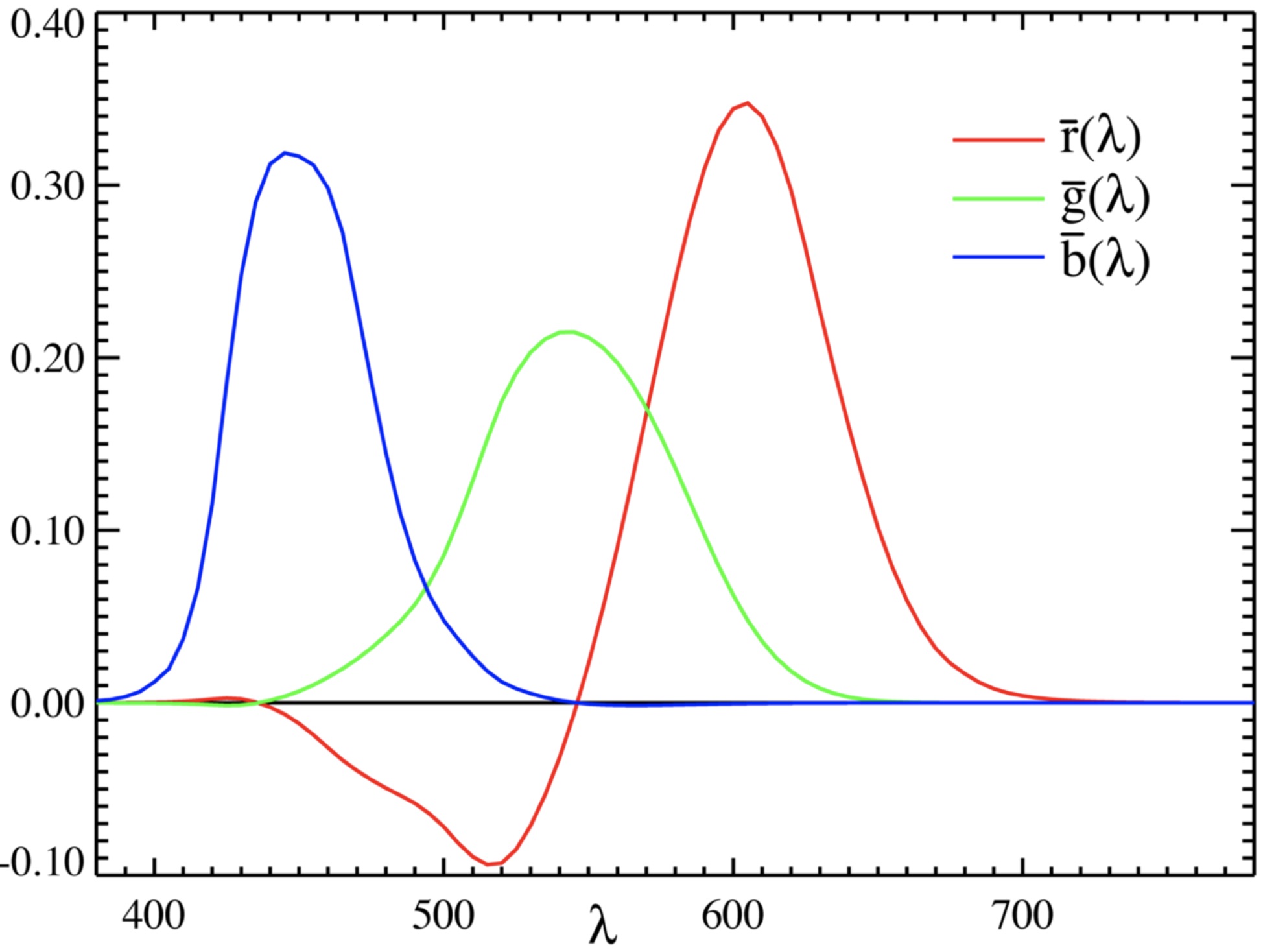
A color space is defined by the matrix, \(\mathbf{C}\), with three rows of color sensitivity functions. These three sensitivity functions, \(\mathbf{C}\), must be some linear combination of the sensitivity functions of the eye, \(\mathbf{C}_{\mbox{eye}}\). One color standard is the Commission Internationale de l’Eclairage (CIE) XYZ color space, \(C_{\mbox{CIE}}\). The CIE color matching functions, the rows of \(\mathbf{C}_{\mbox{CIE}}\) were designed to be all-positive at every wavelength and are shown in Figure 8.13.
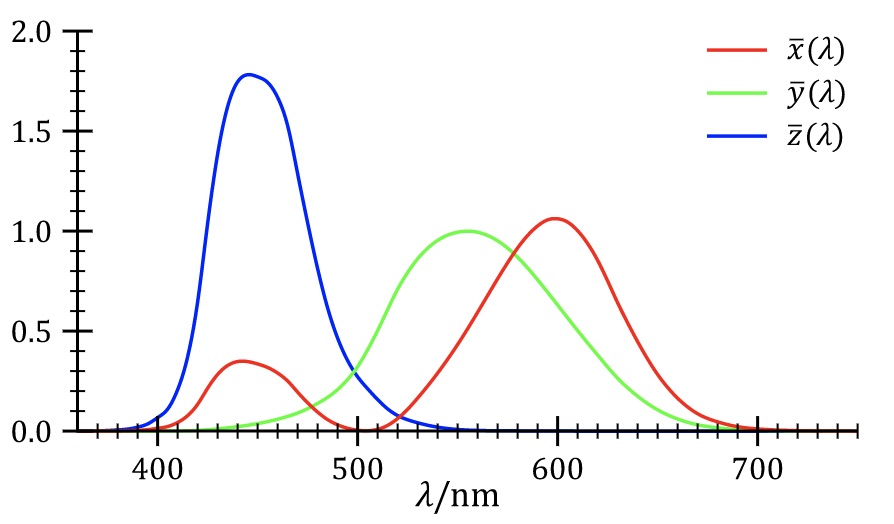
An unfortunate property of the CIE color-matching functions is that no all-positive set of color primaries, \(\mathbf{P}_{\mbox{CIE}}\) forms a color-matching system with those color-matching functions, \(\mathbf{C}_{\mbox{CIE}}\). But \(\mathbf{C}_{\mbox{CIE}}\) is a valid matrix with which to measure colors, even though there is no physically realizable set of corresponding color primaries, \(\mathbf{P}_{\mbox{CIE}}\).
To find the CIE color coordinates, one projects the input spectrum onto the three color-matching functions, to find coordinates, called tristimulus values, labeled \(X\), \(Y\), and \(Z\). Often, these values are normalized to remove overall intensity variations, and one calculates CIE chromaticity coordinates \(x = \frac{X}{X+Y+Z}\) and \(y = \frac{Y}{X+Y+Z}\).
8.4 Spatial Resolution and Color
Color interacts with our perception of spatial resolution. For some directions in color space, the eye is very sensitive to fine spatial modulations, while for other color space directions, the eye is relatively insensitive. Some color coordinate systems take advantage of this disparity to enable efficient representation of images by sampling image data sparsely along color axes where human perception is insensitive to blurring.
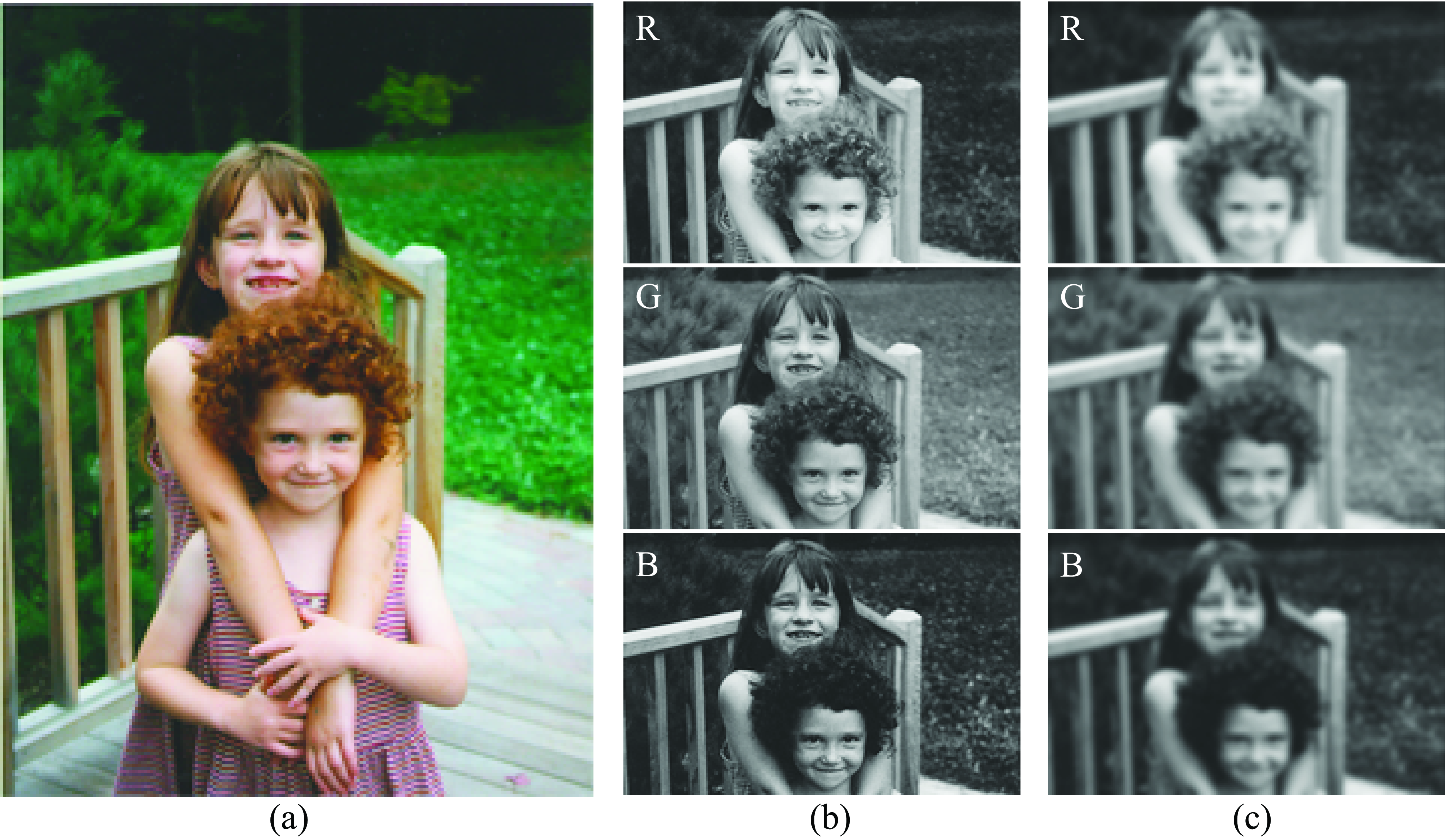
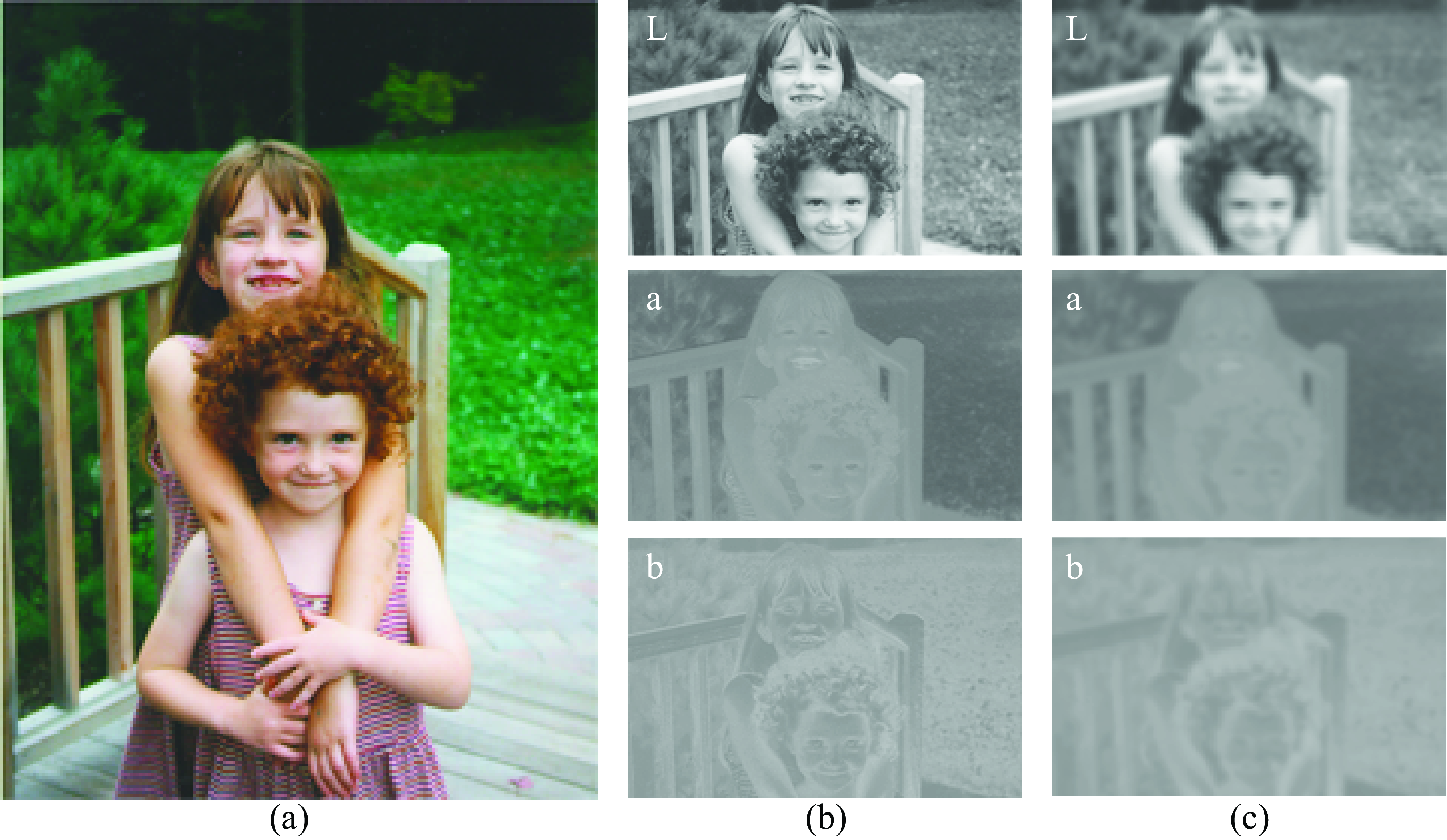
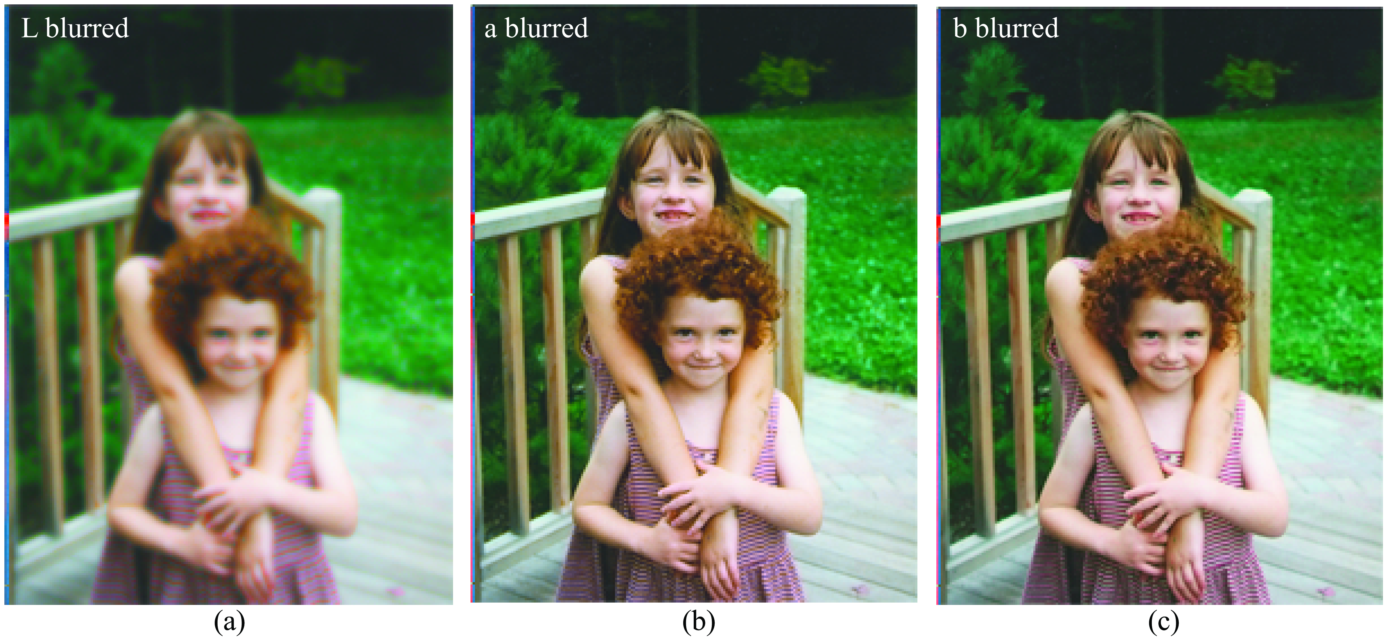
In a red-green-blue (RGB) representation, the eye is sensitive to high spatial frequency changes in both red and green, as shown in figures Figure 8.14 and Figure 8.15. A rotation of the color coordinates of the image, followed by a nonlinear stretching, can put the image into a color space called L, a, b. In that space, the eye is very sensitive to any blurring of the L color component, called luminance, but is relatively insensitive to blurring of the a or b components, as demonstrated in Figure 8.16 and Figure 8.17. This effect is commonly exploited in image compression, allowing some image components to be sampled more coarsely than others.

8.5 Concluding Remarks
The three classes of color sensors in our eyes project light spectra into a 3-dimensional color space. While human perception of color depends on more than just the spectrum of the light being observed, most systems for color matching achieve good results by assuming that the spectrum is all that matters. Linear algebra can find the best controls for a display or printing device in order to match the color measured by a set of sensors.
As would be expected from the spatial varying pattern of color sensors in our eyes–we have few blue or short-wavelength sensors–humans observe different colors with different spatial resolutions, a fact that is exploited in image compression methods.