48 Optical Flow Estimation
48.1 Introduction
Now that we have seen how a moving three-dimensional (3D) scene (or camera) produces a two-dimensional (2D) motion field on the image, let’s see how can we measure the resulting 2D motion field using the recorded images by the camera. We want to measure the 2D displacement of every pixel in a sequence.
Unfortunately, we do not have a direct observation of the 2D motion field either, and not all the displacements in image intensities correspond to 3D motion. In some cases, we can have scene motion without producing changes in the image, such as when the camera moves in front of a completely white wall; in other cases, we will see motion in the image even when there is not motion in the scene such as when the illumination source moves.
In the previous chapter we discussed a matching-based algorithm for motion estimation but it is slow and assumes that the motion is only on discrete pixel locations. In this chapter we will discuss gradient-based approaches that allow for estimating continuous displacement values. These methods introduce many of the concepts later used by learning-based approaches that employ deep learning.
48.2 2D Motion Field and Optical Flow
Before we discuss how to estimate motion, let’s introduce a new concept: optical flow.
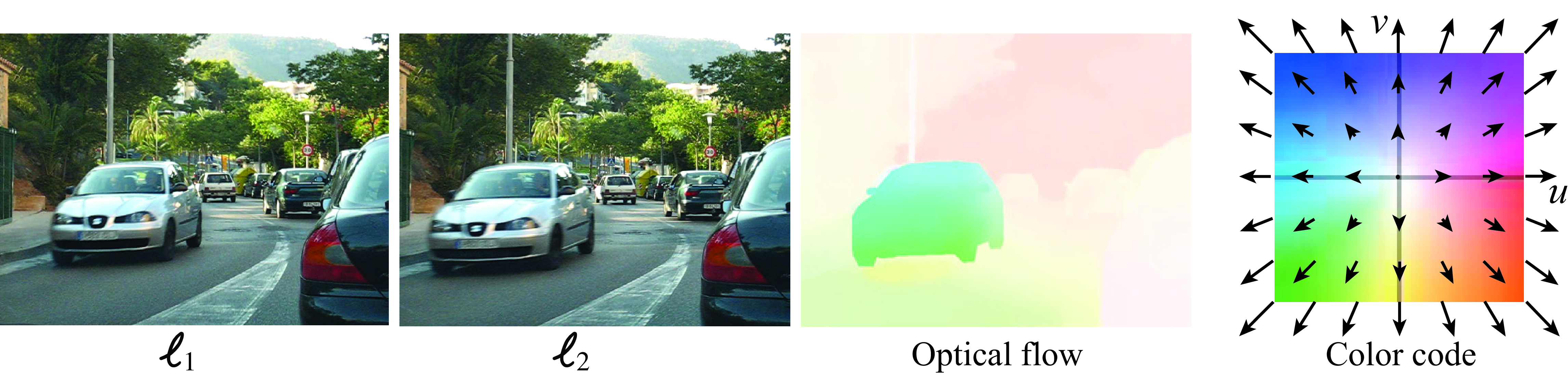
Optical flow is an approximation to the 2D motion field computed by measuring displacement of image brightness (Figure 48.1). The ideal optical flow is defined as follows: given two images \(\boldsymbol\ell_1\) and \(\boldsymbol\ell_2\) \(\in \mathbb{R}^{N \times M \times 3}\), the optical flow \(\left[ \mathbf{u}, \mathbf{v} \right] \in \mathbb{R}^{N \times M \times 2}\) indicates the relative position of each pixel in \(\boldsymbol\ell_1\) and the corresponding pixel in \(\boldsymbol\ell_2\). Note that optical flow will change if we reverse time. This definition assumes that there is a one-to-one mapping between two frames. This will not be true if an object appears in one frame, or when it disappears behind occlusions. The definition also assumes that one motion explains all pixel brightness changes. That assumption can be violated for many reasons, including, for example, if transparent objects move in different directions, or if an illumination source moves.
Figure 48.1 shows two frames and the optical flow between them. This visualization using a color code was introduced in [1]. In this chapter we will use arrows instead as it provides a more direct visualization and it is sufficient for the examples we will work with.
48.2.1 When Optical Flow and Motion Flow Are Not the Same
There are a number of scenarios where motion in the image brightness does not correspond to the motion of the 3D points in the scene. Here there are some examples where it is unclear how motion should be defined:
Rotating Lambertian sphere with a static illumination will produce no changes in the image. If the sphere is static, and the light source moves, we will see motion in spite of the sphere being static.
Moving in front of a textureless wall produces no change on the image.
Waves in water: waves appear to move along the surface but the actual motion of the water is up and down (well, it is even more complicated than that).
A rotating mirror will produce the appearance of a faster motion. And this will happen in general with any surface that has some specular component.
A camera moving in front of a specular planar surface will not produce a motion field corresponding to a homography.
Motion estimation should not just measure pixel motion, it should also try to assign to each source of variation in the image the physical cause for that change. The models we will study in this chapter will not attempt to do this.
48.2.2 The Aperture Problem
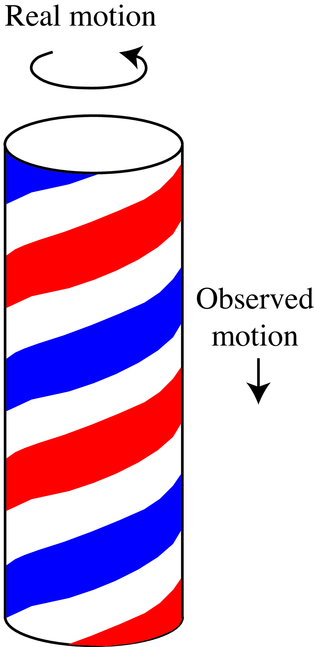
One classical example of the limitations of motion estimation from images is the aperture problem. The aperture problem happens when observing the motion of a one-dimensional (1D) structure larger than the image frame, as shown in Figure 48.2. If none of the termination points are in view within the observation window (i.e., the aperture), it is impossible to measure the actual image motion. Only the component orthogonal to the moving structure can be measured.

The Barber-pole illusion is an illustration of the aperture problem. The barber pole induces the illusion of downward motion while rotating.
48.2.3 Representation of Optical Flow
We can model motion over time as a sequence of dense optical flow images: \[\left[ u(x,y,t), v(x,y,t) \right]\] The quantities \(u(x,y,t)\)and \(v(x,y,t)\) indicate that a pixel at image coordinates \((x,y)\) at time \(t\) moves with velocity \((u,v)\). The problem with this formulation is that we do not have an explicit representation of the trajectory followed by points in the scene over time. As time \(t\) changes, the location \((x,y)\) might correspond to different scene elements.
An alternative representation is to model motion as a sparse set of moving points (tracks): \[\left\{ \mathbf{P}^{(i)}_t \right\}_{i=1}^N\] This has the challenge that we have to establish the correspondence of the same scene point over time (tracking). The appearance of a 3D scene point will change over time due to perspective projection and other variations such as illumination changes over time. It might be difficult to do this on a dense array. Therefore, most representations of motion as sets of moving points use a sparse set of points.
Both of those motion representations have limitations, and depending on the applications, one representation may be preferred over the other. Choosing the right representation might be challenging in certain situations. For instance, what representation would be the most appropriate to describe the flow of smoke or water over time? (We do not know the answer to this question, and the answer might depend on what do we want to do with it.)
In the rest of this chapter we will use the dense optical flow representation.
48.3 Model-Based Approaches
Let’s now describe a set of approaches for motion estimation that are not based on learning. Motion estimation equations will be derived from first principles and will rely on some simple assumptions.
In Section 46.3 we discussed matching-based optical flow estimation. We will discuss now gradient-based methods. These approaches rely on the brightness constancy assumption and use the reconstruction error as the loss to optimize.
48.3.1 Brightness Constancy Assumption
The brightness constancy assumption says that as a scene element moves in the world, the brightness captured by the camera from that element does not change over time. Mathematically, this assumption translates into the following relationship, given a sequence \(\ell(x,y,t)\):
\[\ell(x +u, y+v, t + 1) = \ell(x,y,t) \tag{48.1}\]
where \(u\) and \(v\) are the element displacement over one unit of time and are also a function of pixel location, \(u(x,y)\) and \(v(x,y)\), but we will drop that dependency to simplify the notation. The previous relationship is equivalent to saying that \(\ell(x, y, t + 1) = \ell(x-u,y-v,t)\). To make sure that the reader remains onboard without getting confused by the indices and how the translation works, here is a simple toy example of a translation with \((u=1, v=0)\):
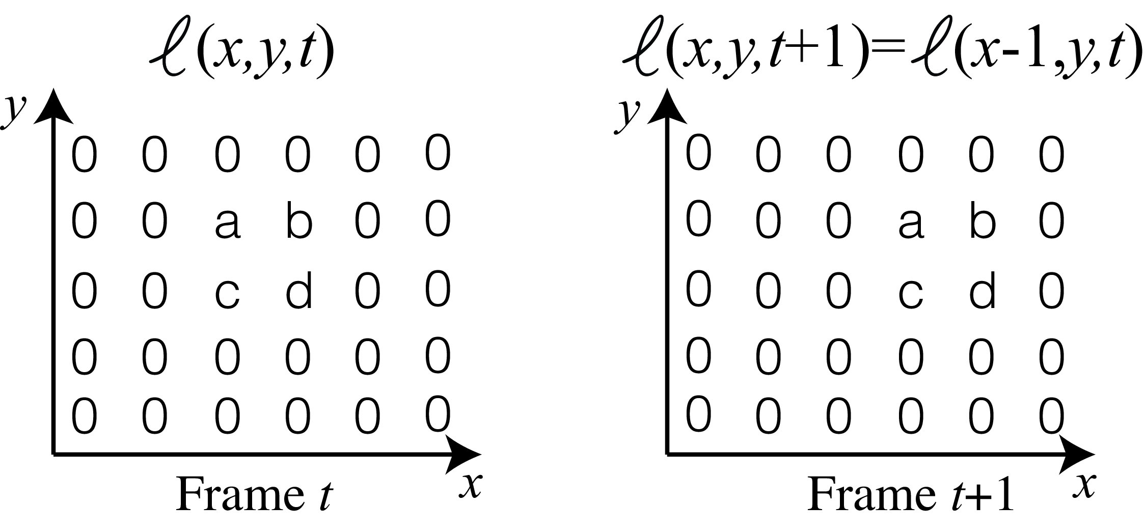
The constant brightness assumption only approximately holds in reality. For it to be exact, we should have a scene with Lambertian objects illuminated from a light source at infinity, with no occlusions, no shadows, and no interreflections. Few real scenes check any of those boxes. This equation assumes that all the pixels in \(\ell(x, y, t)\) are visible in \(\ell(x, y, t+1)\), but in reality, some pixels might be occluded in the first frame and new pixels might appear around the image boundaries and behind occlusions.
48.3.2 Gradient-Based Optical Flow Estimation
The most popular version of a gradient-based method for optical flow estimation was introduced by Lucas and Kanade in 1981 [2].
Let’s start describing the method in words, and we will see next how it translates into math. We will start by approximating the change between two consecutive frames by a linear equation using a Taylor approximation. This linear approximation combined with the constant brightness assumption will result in a linear constraint for the optical flow at each pixel. We will then derive a big system of linear equations for the entire image that, when solved, will result in an estimated optical flow for each image pixel. Let’s now see, step by step, how this algorithm works.
If the motion \((u,v)\) is small in comparison to how fast the image \(\ell\) changes spatially, we can use a first-order Taylor expansion of the image \(\ell(x +u, y+v, t + 1)\) around \((x,y,t)\): \[\ell(x +u, y+v, t + 1) \simeq \ell(x,y,t) + u \ell_x + v \ell_y + \ell_t + \mbox{h. o. t.} \tag{48.2}\]
Combining equations (Equation 48.1) and (Equation 48.2), and ignoring higher order terms, we arrive at the gradient constraint equation: \[u \ell_x + v \ell_y + \ell_t = 0\]This equation constrains the motion \((u,v)\) in location \((x,y)\) to be along a line perpendicular to the image gradient \(\nabla \ell= \left( \ell_x, \ell_y \right)\) at that location. This is the same relationship that we discussed before when describing the aperture problem. This is not enough to estimate motion and we will need to add additional constraints. The second assumption that we will add is that the motion field is constant (or smoothly varying) over an extended image region. By solving for the gradient constraints over an image patch, we hope there will be only a unique velocity that will satisfy all the equations. We can implement this constraint in a different way. One simple way of implementing this constraint is by summing over a neighborhood using a weighting function \(g(x,y)\). If \(g(x,y)\) is a Gaussian window centered in the origin, the optical flow, \((u,v)\), at the location \((x,y)\) can be estimated by minimizing: \[\mathcal{L}(u, v) = \sum_{x',y'} g(x'-x,y'-y) \left| u(x,y) \ell_x (x',y',t) + v(x,y) \ell_y(x',y',t) + \ell_t(x',y',t) \right| ^2\] The previous equation is a bit cumbersome because we wanted to make explicit the spatial variables, \((x',y')\), over which the sum is being made and the factors that are function of the location \((x,y)\) at which the flow is computed. From now, to simplify the derivation, we will drop all the arguments and write the loss in a single location as:
\[ \mathcal{L}(u, v) = \sum g \left| u \ell_x + v \ell_y + \ell_t \right| ^2 \] where only \(u\) and \(v\) are constant.
The solution that minimizes this loss can be obtained by computing where the derivatives of the loss with respect to \(u\) and \(v\) are equal to zero:
\[\begin{aligned} \frac{\partial \mathcal{L}(u, v)}{\partial u } = \sum g \left( u \ell_x ^ 2 + v \ell_x \ell_y + \ell_x \ell_t \right) = 0 \\ \frac{\partial \mathcal{L}(u, v)}{\partial v } = \sum g \left( u \ell_x \ell_y + v \ell_y^2 + \ell_y \ell_t \right) = 0 \end{aligned}\]
We can write the previous two equations in matrix form at each location \((x',y')\) as:
\[\begin{bmatrix} \sum g \ell_x ^ 2 & \sum g \ell_x \ell_y \\ \sum g \ell_x \ell_y & \sum g \ell_y ^ 2 \end{bmatrix} \begin{bmatrix} u \\ v \end{bmatrix} = - \begin{bmatrix} \sum g \ell_x \ell_t \\ \sum g \ell_y \ell_t \end{bmatrix} \tag{48.3}\]
We will have an equivalent set of equations for each image location. The solution at each location can be computed analytically as \(\mathbf{u} = \mathbf{A}^{-1} \textbf{b}\) where \(\mathbf{A}\) is the \(2 \times 2\) matrix of equation (Equation 48.3). The motion at location \(x,y\) will only be uniquely defined if we can compute the inverse of \(\mathbf{A}\). Note that the matrix \(\mathbf{A}\) is a function of the image structure around location \((x,y)\). If the rank of the matrix is 1, we can not compute the inverse and the optical flow will be constrained along a 1D line, this is the aperture problem. This will happen if the image structure is 1D inside the region of analysis that will be defined by the size of the Gaussian window \(g(x,y)\).
In order to implement this approach we can make use of convolutions in order to compute all the quantities efficiently in a compact algorithm Algorithm 48.1:
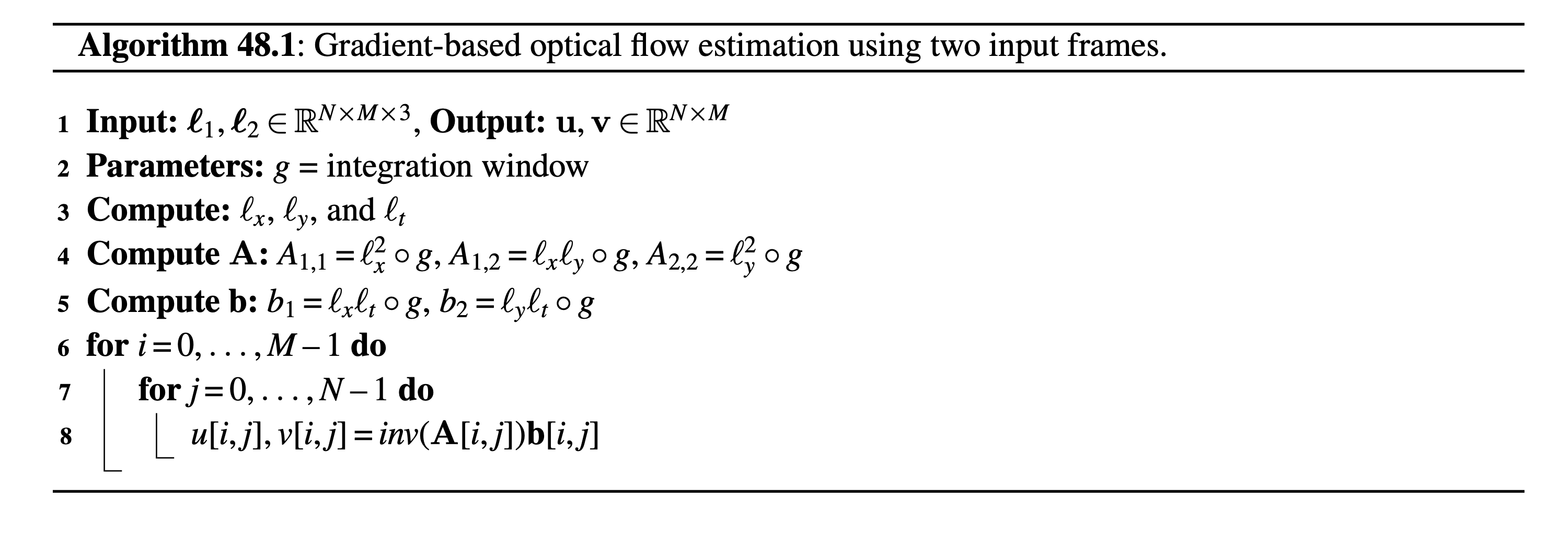
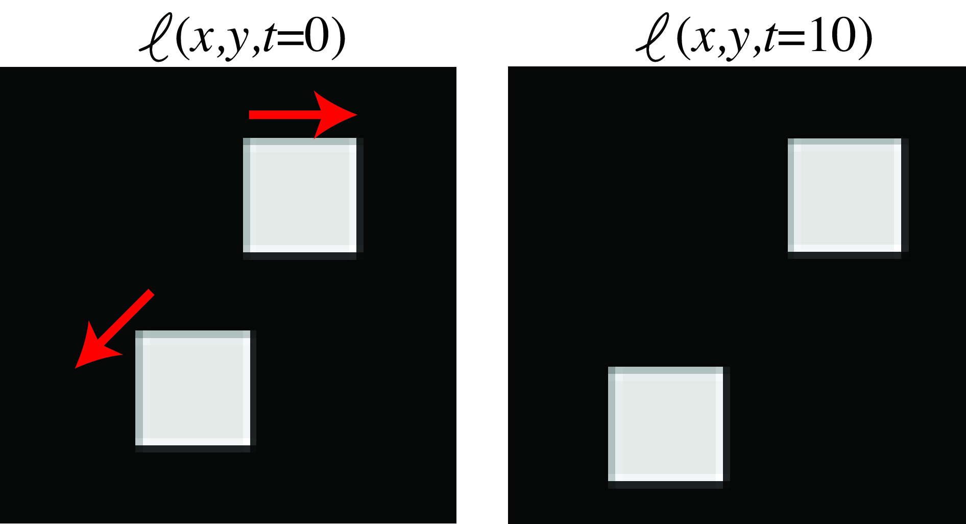
To see how optical flow is computed from gradients, let’s consider a simple sequence with two moving squares as shown in Figure 48.4 where the top square moves with a velocity of \((0,0.5)\) pixels/frame and the bottom one moves at \((-0.5, -0.5)\) pixels/frame (the figure shows frames \(0\) and \(10\) to make the motion more visible).
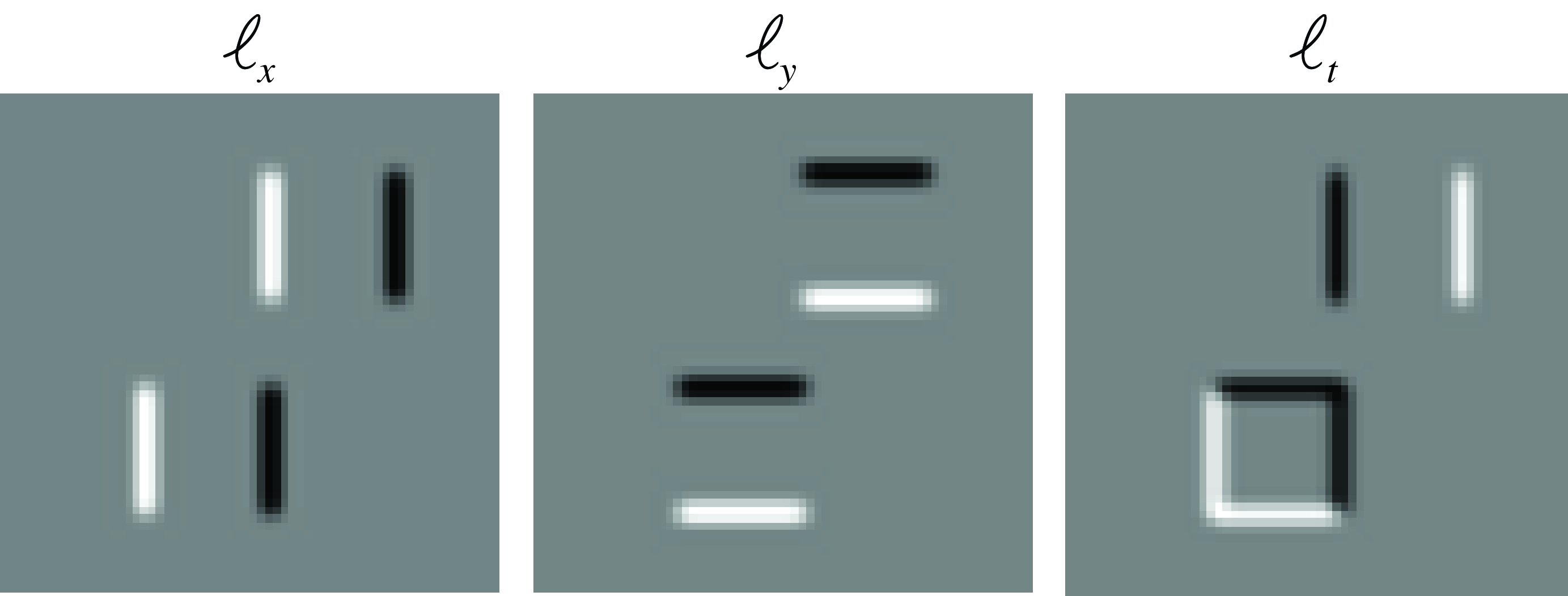
To apply the gradient-based optical flow algorithm we need to compute the gradients along \(x\), \(y\), and \(t\). In practice, the image derivatives, \(\ell_x\) and \(\ell_y\), are computed by convolving the image with Gaussian derivatives (see Chapter 18). In the experiments here we first blur the two input frames with a Gaussian of \(\sigma=1\), approximated with a five-tap kernel (i.e., a kernel with size \(5 \times 5\) values). For the spatial derivatives we use the kernel \([1, -8, 0, 8, -1]/12\) for the \(x\)-derivative and its transposed for the \(y\)-derivative. The temporal derivative can be computed as the difference of two consecutive blurred frames. Choosing the appropriate filters to compute the derivatives is critical to get correct motion estimates (the three derivatives need to be centered at the same spatial and temporal location in the \(x-y-t\) volume). For the moving squares sequence, the spatial and temporal derivatives are shown in Figure 48.5.
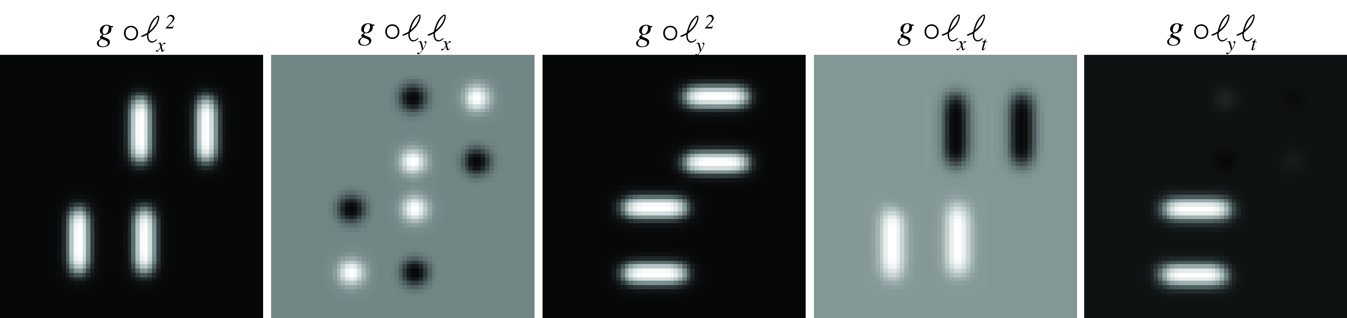
The next step consists of computing \(\ell_x^2\), \(\ell_x\ell_y\), \(\ell_y^2\), \(\ell_x\ell_t\), and \(\ell_y\ell_t\) and blurring them with the Gaussian kernel, \(g\), which will then be used to build the matrix \(\mathbf{A}\) at each pixel. Figure 48.6 shows the results.
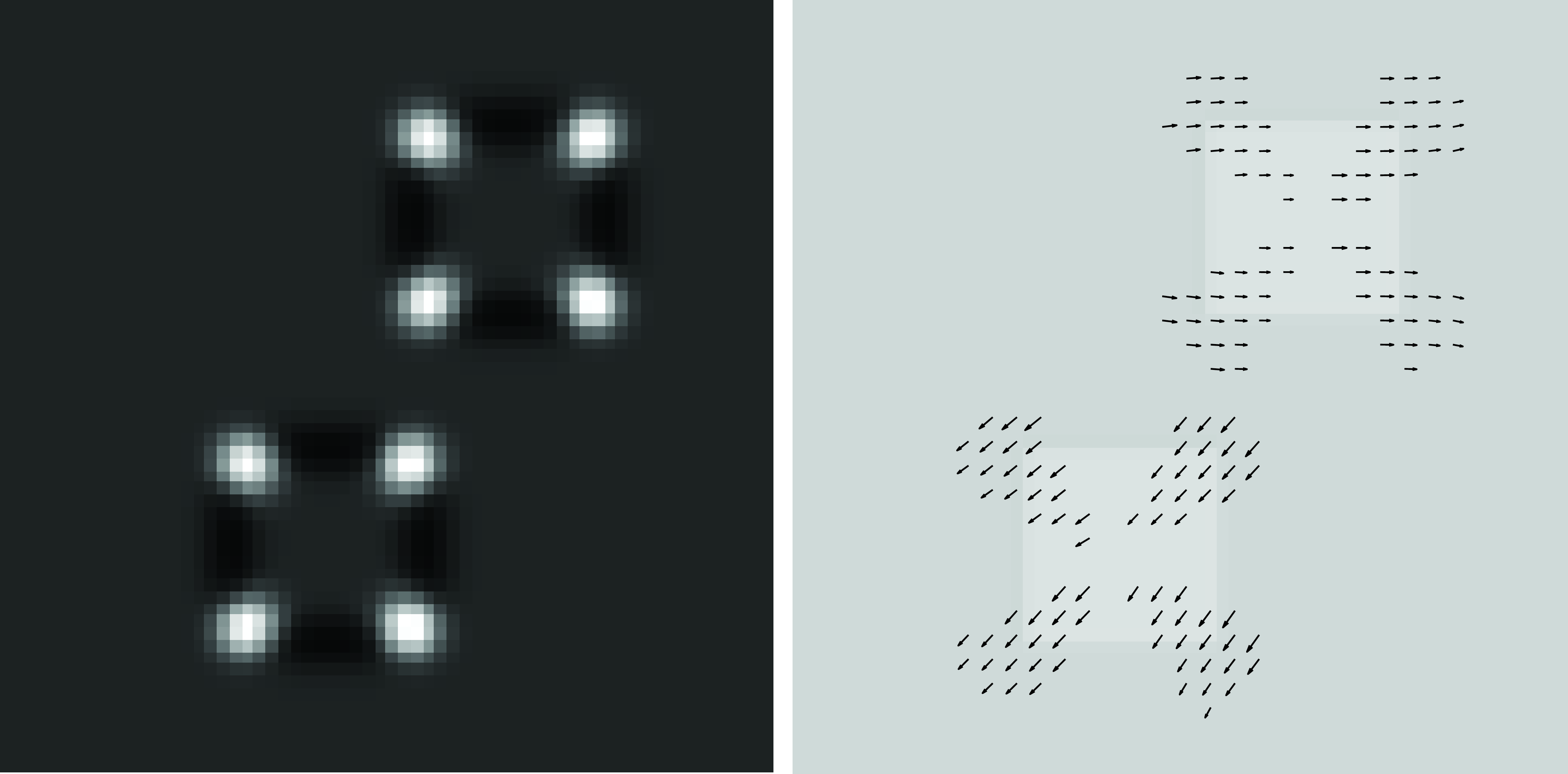
In order to compute the optical flow, we need to compute the matrix inverse \(\mathbf{A}^{-1}\). This matrix depends only on the spatial derivatives and thus is independent of the motion present in the scene. If we compute optical flow at each pixel, the result looks like the image in Figure 48.7.

We can see that the result seems to be wrong for the motion estimated near the center of the side of each square. The inverse can only be computed in image regions with sufficient texture variations (i.e., near the corners). As in the Harris corner detector (see Section 40.3.2.1), the eigenvector with the smallest eigenvalue indicates the direction in which the image has the smallest possible change under translations. Regions with a small minimum eigenvalue are regions with a 1D image structure and will suffer from the aperture problem. To identify regions where the motion will be reliable, we can use the following quantity (proposed by Harris), which relates to the conditioning of the matrix \(\mathbf{A}\): \[R = \det (\mathbf{A}) - \lambda \mathrm{Tr}\hspace{1pt} (\mathbf{A})^2\]where \(\lambda=0.05\) (which is within the range of values used in the Harris corner detector). Figure 48.8 shows \(R\) and the estimated optical flow in the regions with \(R > 2\). Harris proposed this formulation to avoid the computation of the eigenvalues at each pixel because it is computational expensive.
The regions for which \(R > 2\) will increase by making the apertures larger, which is achieved by using a Gaussian filter, \(g\), with larger \(\sigma\). However, this will result in smoother estimated flows and the estimated motion will not respect the object boundaries.
One advantage of this approach over the matching-based algorithm is that the estimated flow is not discrete, but it does not work well if the displacement is large, as the Taylor approximation is not valid anymore. One solution to the problem of large displacements is to compute a Gaussian pyramid for the input sequence. The low-resolution scales make the motion smaller and the gradient-based approach will work better.
48.3.3 Iterative Refinement for Optical Flow
The gradient-based approach is efficient but it only provides an approximation to the motion field because it ignores higher order terms in the Taylor expansion in equation (Equation 48.2). A different approach consists of directly minimizing the photometric reconstruction error: \[L(\boldsymbol\ell_1,\boldsymbol\ell_2,\mathbf{u}, \mathbf{v})= \sum_{x,y} \left| \ell_1 (x+u,y+v,t+1) - \ell_2 (x,y,t)) \right| ^2\]
We can now run gradient descent on this loss. Running only one iteration would be similar to the gradient-based optical flow algorithm described in the previous section. However, adding iterations will provide a more accurate estimate of optical flow. At each iteration \(n\), the estimated optical flow will be used to compute the warped frame \(\ell_1 (x+u_n,y+v_n,t+1)\) and we will compute an update, \(\Delta u_n\) and \(\Delta v_n\), of the optical flow: \(u_{n+1} = u_n+\Delta u_n\) and \(v_{n+1}= v_n + \Delta v_n\). To improve the results, the optical flow estimation is done on a Gaussian pyramid. First, we run a few iterations on the lowest resolution scale of the pyramid (where the motion will be the smallest). The estimated motion is then upsampled and used as initialization at the next level. We iterate this process until arriving at the highest possible resolution. This process is shown in Figure 48.9.
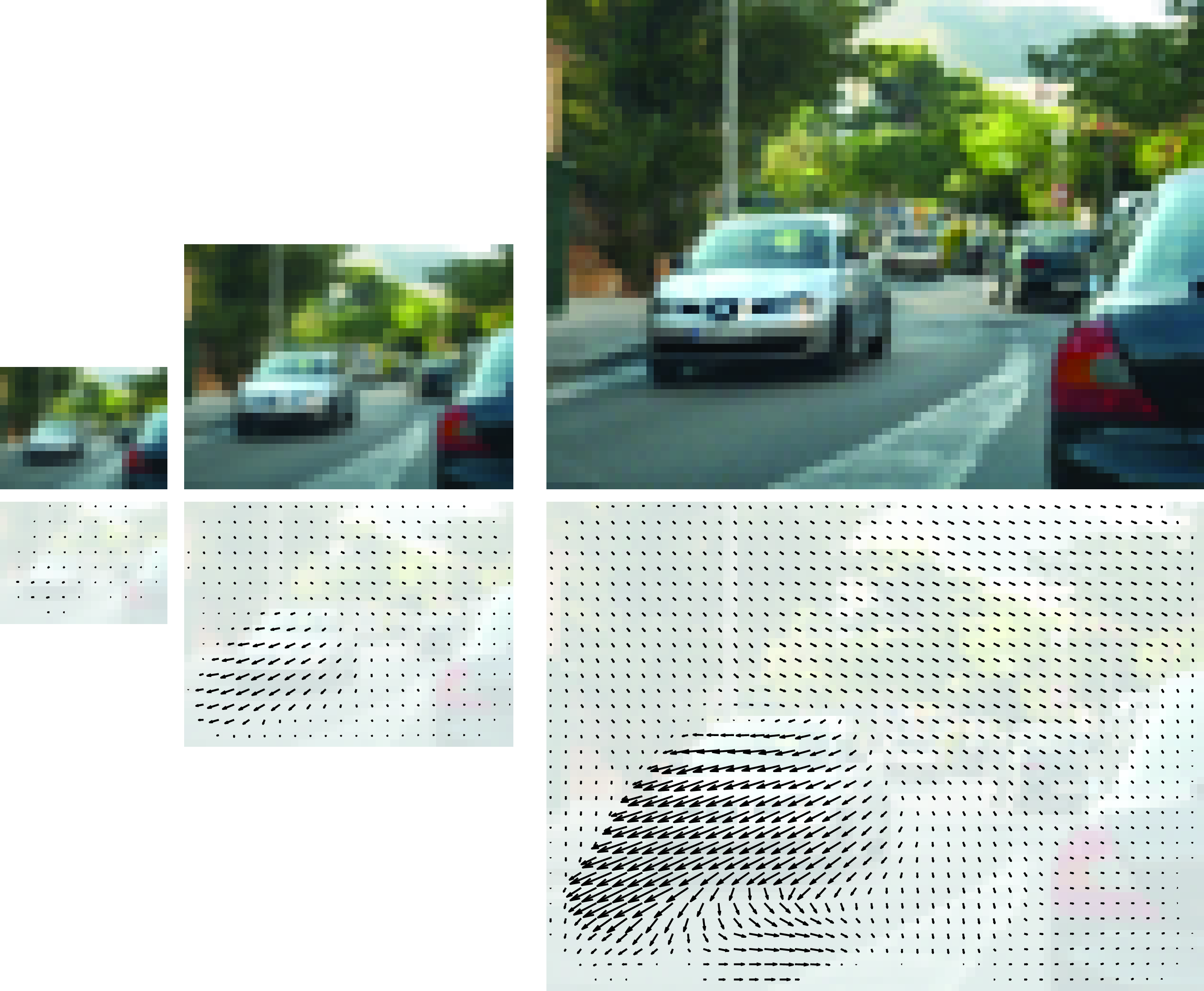
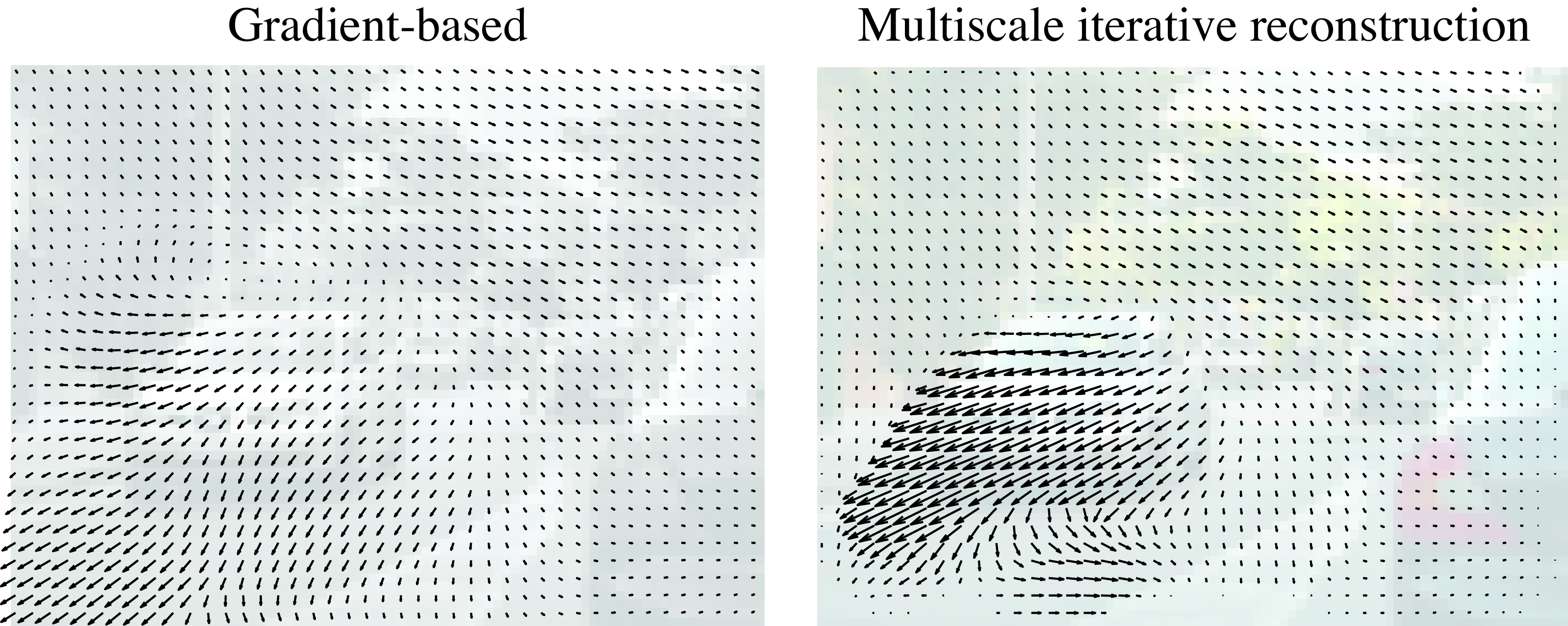
Figure 48.10 compares the optical flow computed using the gradient-based algorithm (i.e., one iteration) and the multiscale iterative refinement approach. Note how the gradient-based approach underestimates the motion of the left car. The displacement between consecutive frames is close to four pixels and that makes the first-order Taylor approximation very poor. The multiscale method is capable of estimating large displacements.
The photometric reconstruction can incorporate a regularization term penalizing fast variations on the estimated optical flow: \[ \mathcal{L}(\mathbf{u}, \mathbf{v}) = L(\boldsymbol\ell_1,\boldsymbol\ell_2,\mathbf{u}, \mathbf{v}) + \lambda R(\mathbf{u}, \mathbf{v}) \\ \tag{48.4}\] This problem formulation was introduced by Horn and Schunck in 1981 [4].
There are several popular regularization terms. One penalizes large velocities (slow prior):
\[ R(\mathbf{u}, \mathbf{v}) = \sum_{x,y} \left( u(x,y) \right)^2 + \left( v(x,y) \right)^2 \]
Another penalizes variations on the optical flow (smooth prior): \[R(\mathbf{u}, \mathbf{v}) = \sum_{x,y} \left( \frac{\partial u}{\partial x} \right)^2 + \left( \frac{\partial u}{\partial y} \right)^2 + \left( \frac{\partial v}{\partial x} \right)^2 + \left( \frac{\partial v}{\partial y} \right)^2\]
The photometric loss plays an important role in unsupervised learning-based methods for optical flow estimation as we will discuss later.
48.3.4 Layer-Based Motion Estimation
Until now we have not made use of any of the properties of the motion field derived from the 3D projection of the scene. One way of incorporating some of that knowledge is by making some strong assumptions about the moving scene. If the scene is composed of rigid objects, then we can assume that the motion field within each object will have the form described by equation (Equation 47.8).
In this case, instead of a moving camera we have rigid moving objects (which is equivalent). The 2D motion field can then be represented as a collection of superimposed layers, each layer containing one object and occluding the layers below. Each layer will be described by a different set of motion parameters. The parametric motion field can be incorporated into the gradient-based approach described previously. The motion parameters can then be estimated iteratively using an expectation-maximization (EM) style algorithm. At each step we will have to estimate, for each pixel, which layer it is likely to belong to, and then estimate the motion parameters of each layer. The idea of using layers to represent motion was first introduced by Wang and Adelson in 1994 [5].
48.4 Concluding Remarks
Motion estimation is an important task in image processing and computer vision. It is used in video denoising and compression. In computer vision it is a key attribute to understand scene dynamics and 3D structure. Despite being studied for a long time, accurate optical flow remains challenging, even when using state-of-the-art deep-learning techniques.
The approaches presented here require no training. In the next chapter, we will study several learning-based methods for motion estimation. The approaches presented in this chapter will become useful when exploring unsupervised learning methods.