31 Perceptual Grouping
31.1 Introduction
The previous chapter discussed the importance of learning good visual representations, which can serve as the substrate for further vision algorithms. In this chapter we will continue our exploration of perceptual representations, but we will approach it from a slightly different school of thought, which is inherited from pre-deep learning computer vision and from human vision science. In this tradition, one particular kind of visual representation, the perceptual group, becomes the central object of interest; we will see what these are, how to find them, and how they are related to the representation learning algorithms from the last chapter.
First, what is a perceptual group? Look at the photo in Figure 31.1 and consider what you see. Not what raw pixel values you see, but what structures you see. What are some structures you can name?

What a camera sees is the raw RGB pixel values of the photo. But what your mind sees is rather different. You see contours and surfaces, objects and events.
Many of these perceptual structures can be thought of as groups of primitive elements: a contour is a group of points that form a line, an object is a group of parts that form a cohesive whole, and so on. Because of this, understanding how humans, and machines, can identify meaningful perceptual groups has been a longstanding area of interest in both human and computer vision [1].
The content of this chapter can also go under the name perceptual organization, which is the study of how our vision system organizes the pixels into more abstracted structures, such as perceptual groups. The Gestalt psychologists were some of the first to study this problem [2].
This leads us to a central question: which primitives should be grouped? We will examine a few answers below, including the idea that primitives should be grouped based on similarity or based on association. We will also look at how natural groups can emerge as a byproduct of a downstream purpose.
31.2 Why Group?
Grouping is a special case of representation learning, and the reasons to group are the same as the reasons to do representation learning: groups are a good substrate for downstream analysis and processing. To get an intuition for why this is, consider how you might describe the scene around you. Go ahead and write down what you see. If you are in a cafe, you might write, “I’m sitting at a table with my laptop in front of me. A latte is next to the laptop; the foam and coffee are swirling into a spiral.”
Now let’s look at each of these words. Some refer to objects (e.g., “table”, “laptop”, “latte”). Others refer to spatial relationships (“in front”, “next to”), and still others refer to shapes (“spiral”) and events (“swirling”). These kinds of structures—objects, relationships, shapes, events—are the elements of perceptual organization, and you can think of perceptual organization as being a lot like describing an image in text. One of the hottest current trends in computer vision is to map images to text, then use the tools of natural language processing to reason about the image content. In this way text is treated as a powerful image representation, and indeed it has become clear that this kind of image representation—symbolic, discrete, semantic—can be exceedingly effective [3], [4], [5], [6].
Perceptual organization is all about trying to get similarly powerful representations, but doing so via bottom-up grouping rules, rather than by mimicking human language. In other words, perceptual organization is about discovering language-like structures in the first place, from unsupervised principles rather than from human-language supervision. Why do we have the words we have, where did they come from? What exactly is an object? This chapter may start to provide some answers.
Although the analogy to text makes clear why perceptual organization is important, perceptual groups can also go beyond the limits of language. Some structures we see are hard to name but still clearly represent a coherent group in our heads. Consider, for example, the image in Figure 31.2 below.

There are clearly two separate objects, but we don’t have names for them. The next sections will cover a few different kinds of perceptual groups that are important in vision.
31.3 Segments
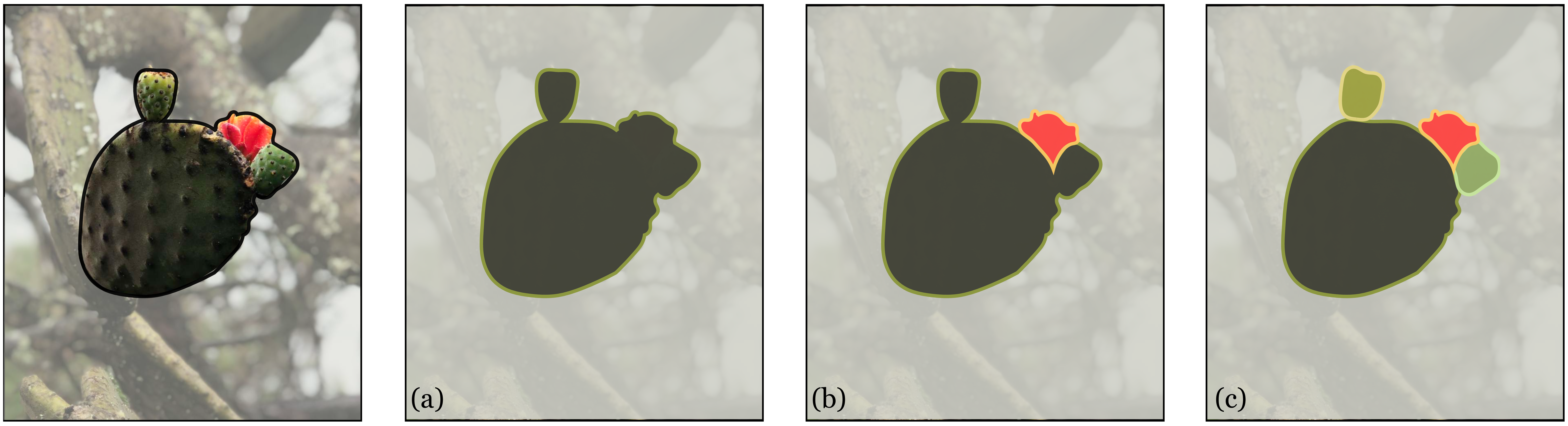
Segmentation is the problem of partitioning an image into regions that represent different coherent entities. There is no single definition of what is a coherent entity and it will vary depending on the task; a segment could correspond to a nameable object, or a image region made of a single material, or a physically distinct piece of geometry (see Figure 31.3).
Segmentation can be framed as a clustering problem: assign each pixel in an image to one of \(k\) clusters. We will explore two approaches to solving this clustering problem: (1) assign similar pixels to the same cluster, (2) assign two pixels to the same cluster if there is no boundary between them. We will start with the first.
31.3.1 \(K\)-Means Segmentation
\(K\)-means, which we covered in Chapter 30, is one of the simplest and most useful clustering algorithms, so let’s try it for segmentation.
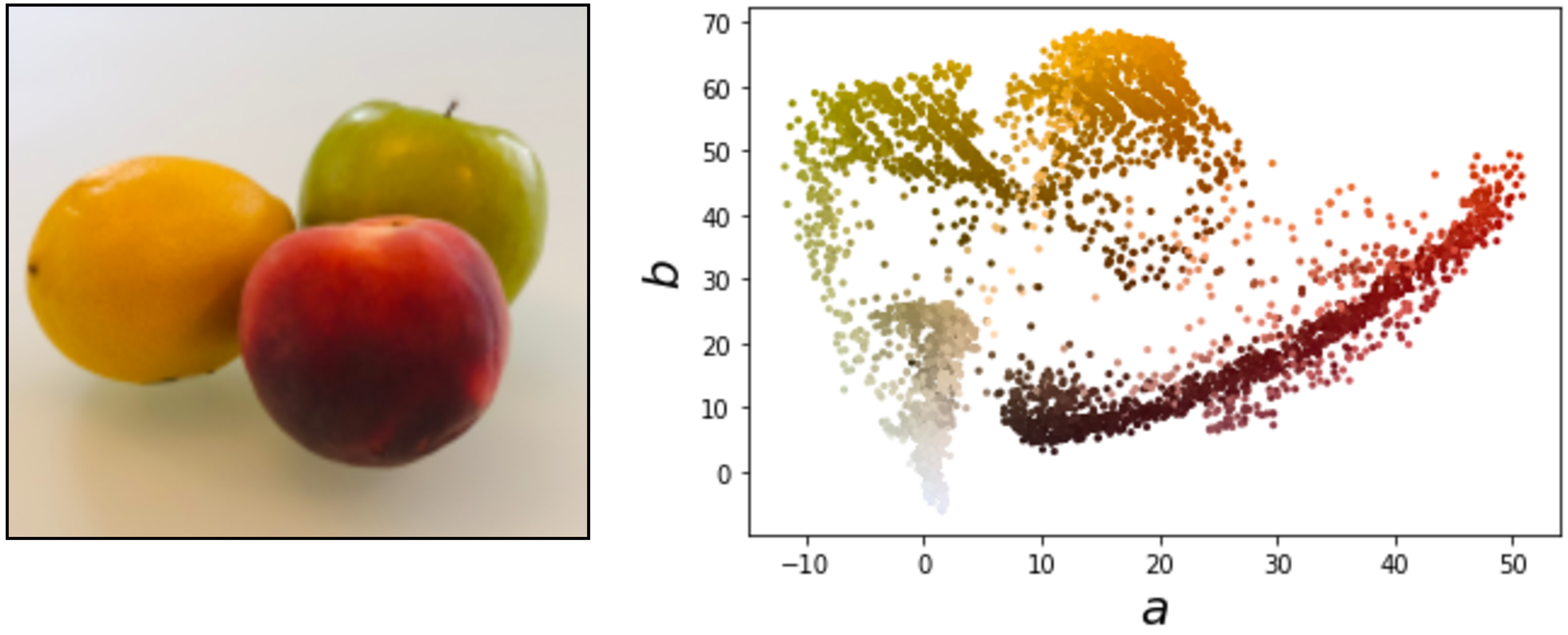
\(K\)-means operates on a data matrix of \(N\) datapoints by \(M\) features per datapoint. Our first task is to convert the segmentation problem to that format. The simplest thing to do is let each pixel be a datapoint and the pixel’s color be its feature vector. For ease of visualization, we will use the \(ab\) color value as the two-dimensional (2D) feature per pixel. An image represented this way can be plotted as a scatter plot and you can think of it as samples from a distribution over \(ab\) colors, as shown in Figure 31.4.
\(K\)-means tries to find clusters in this scatter plot (and, if you prefer a probabilistic interpretation, it can be thought of as fitting a mixture of Gaussians to the datapoints, which aims to approximate the distribution from which these pixels were sampled). We can segment via \(k\)-means by simply assigning each pixel to the cluster assignment of its color value. Below we color each pixel in each cluster by the mean color of all pixels assigned to that cluster (Figure 31.5).
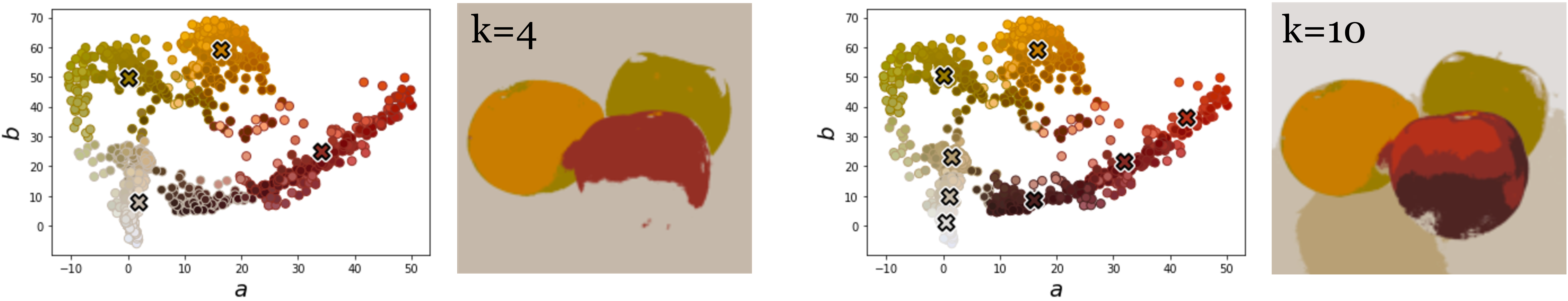
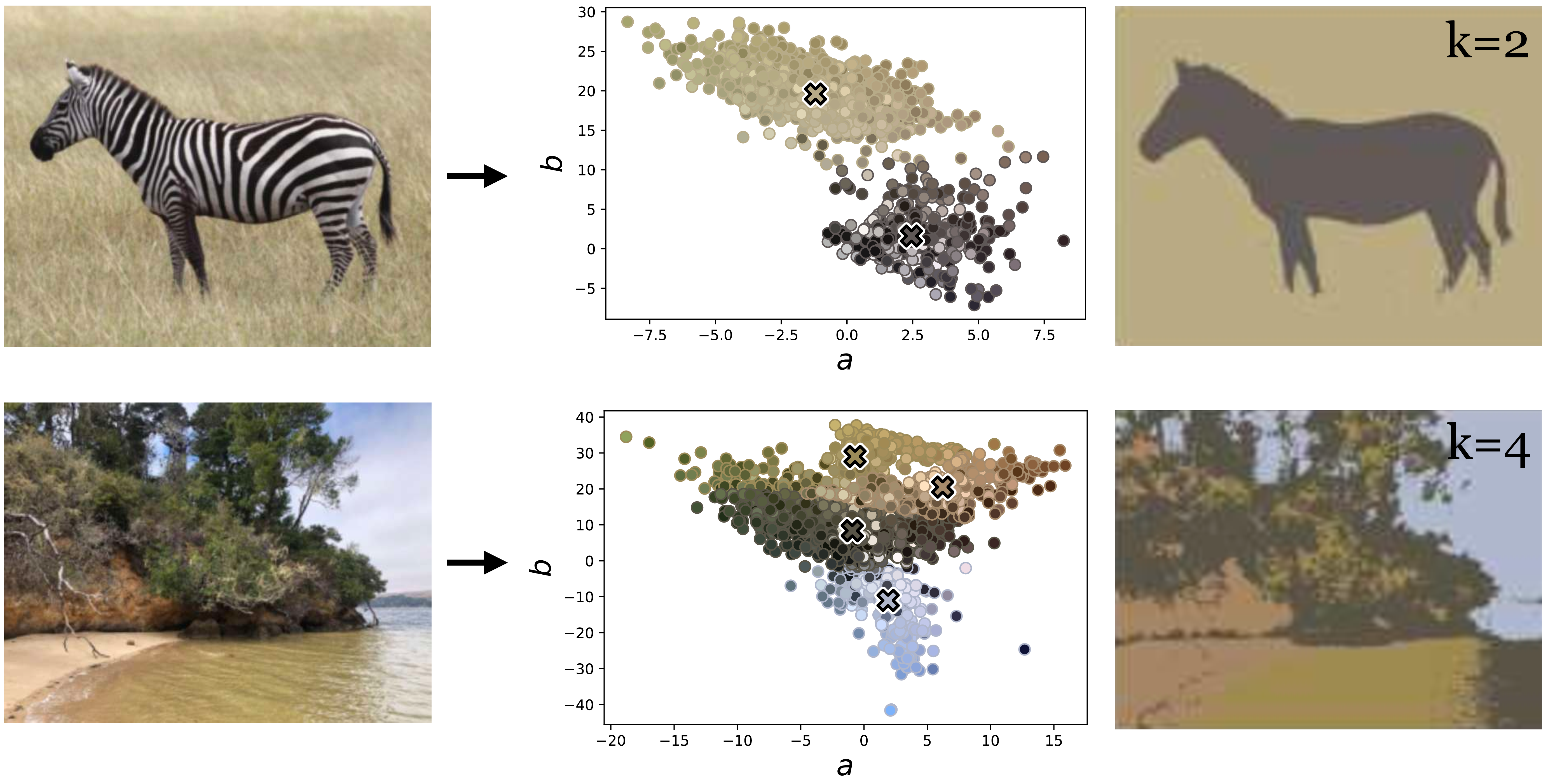
Naturally, \(k\)-means on \(ab\)-values finds segments that correspond to regions of roughly a constant color. This simple approach can be surprisingly effective. Notice how it segments a zebra from the background in Figure 31.6 (because the black and white stripes have roughly the same \(ab\)-values). However, it fails to group more complex patterns that are not defined by color similarity, as in the beach photo in Figure 31.6.
31.3.2 Affinity-Based Segmentation
Other clustering methods are based on the idea of affinity, where we try to model a distance metric (the affinity) that tells us whether two items should be grouped. The distance metric usually measures how similar two patterns are, or how likely they are to be part of the same object.
For example, a simple affinity function over pixel pairs could just be the Euclidean distance between the color values of the two pixels. There are numerous ways we could use such an affinity to group pixels into segments, all of which share the general idea that pixels with high affinity should belong to the same group and pixels with low affinity should belong to two different groups. Methods that use this idea include those based on graph cuts [7], spectral clustering [8], and Markov random field (MRF)-based clustering (Chapter 29).
We do not have time to cover all these methods and in fact they are no longer commonly used. Instead we will focus on a method you have seen earlier in the book that actually is in common use: contrastive learning (which was covered in Section 30.10). Contrastive learning is a perfect fit for affinity-based segmentation because contrastive methods learn from similarities (positive pairs) and differences (negative pairs), and this is what an affinity metric gives us! Contrastive methods learn an embedding in which datapoints with high affinity are nearby and datapoints with low affinity are far apart. Once we have such an embedding, clustering is easy in the embedding space, and pretty much any off-the-shelf clustering algorithm will work; for simplicity, we will stick with \(k\)-means in this book.
In this book we only present one way to do affinity-based clustering: first use affinities to supervise a embedding in which the data is nearly clustered, then read off the clusters using a simple quantization method like \(k\)-means. There are many other affinity-based methods but this simple method often works well.
If we define affinities in terms of color distance, then there’s no point in learning such an embedding, because the raw colors themselves are already a great embedding under that notion of affinity. Affinity-based clustering only really becomes interesting when we have nontrivial affinities to model; for example, they could be given by human judgments about which pixels should go together in natural images.
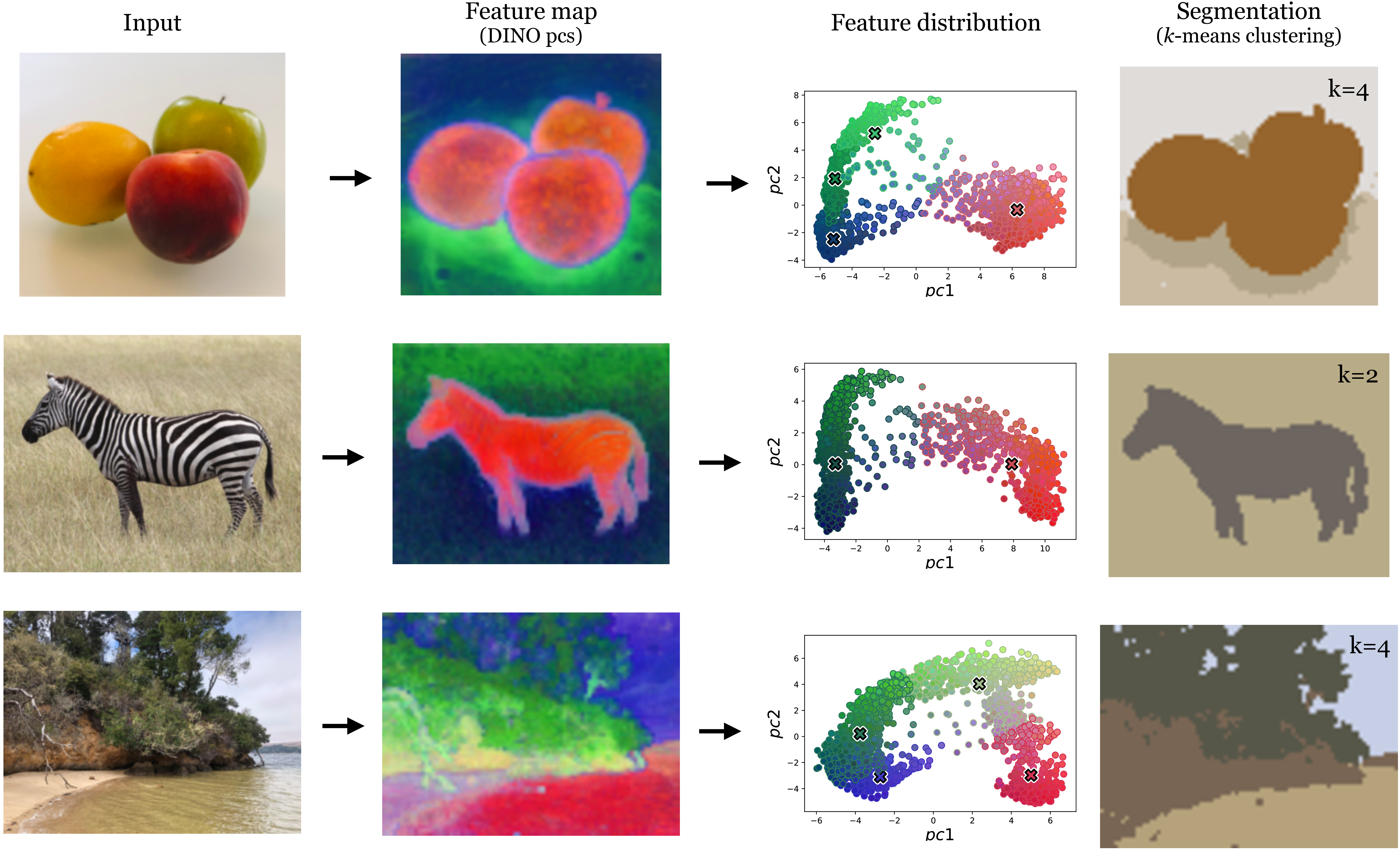
Because human supervision is expensive and limiting, a popular alternative is to use self-supervised affinity measures, just like we saw in self-supervised contrastive learning. Popular contrastive learning methods like SimCLR [9], MoCo [10], and DINO [11], train a mapping from image patches to embedding vectors such that two patches that come from the same image embed near each other and patches from different images embed far apart. We can run these methods densely (in a sliding window fashion) across a single image to create a feature map of size \(C \times N \times M\), where \(N\) and \(M\) are the spatial dimensions of the feature map and \(C\) is the dimensionality of the embedding vectors. This creates a new image where each pixel has a value (the embedding vector) that is similar to other pixels that the model thinks would be likely to appear in the same scene. In effect, we have learned an affinity metric based on natural patch co-occurrences, then used that affinity metric to obtain a feature map that reveals the coherent regions of an image. If we apply \(k\)-means to the pixels in this feature map, we can obtain an effective segmentation. This entire pipeline is shown in Figure 31.7, using DINO [11] as the particular contrastive embedding.
31.4 Edges, Boundaries, and Contours
A complementary problem to segmentation is boundary detection, because a partitioning of an image can be represented either by partition assignments (segments) or by the boundaries between partitions. Many vision algorithms organize images into different kinds of boundaries between perceptual structures. Early vision algorithms focused on edge detection, where the idea was that the edges in an image should form a good, compact representation of the image’s content, because edges are relatively sparse, and they are stable with respect to nuisances like noise and lighting. Subsequent work identified connections between different kinds of edge structure and scene geometry; for example, an edge that represents an occluding contour indicates that there is a depth discontinuity at that location in the scene.
Chapter 2 described some simple edge detectors and showed their use in reconstructing scene geometry. Chapter 42 covers more recent approaches to inferring three-dimensional (3D) scene structure, which have largely superseded the methods that explicitly reasoned about edges.
Line drawings are another way of representing the edge structure in an image, and they seem to be of high interest to humans. This suggests that there may be something useful about representing images in terms of their edge structure. Although there is an active line of research in computer graphics on modeling line drawings, this work has not yet paid off in vision, and it remains unclear whether or not line drawings will one day prove as compelling to visually intelligent machines as they do to us humans.
31.5 Layers
If you have ever seen an early Disney cartoon (e.g., Snow White), you may have noticed a compelling illusion of depth created by parallax between different layers of the animated scene.
An schematic of a multiplane camera from William E. Garity’s 1940 patent for a “Control Device for Animation.” 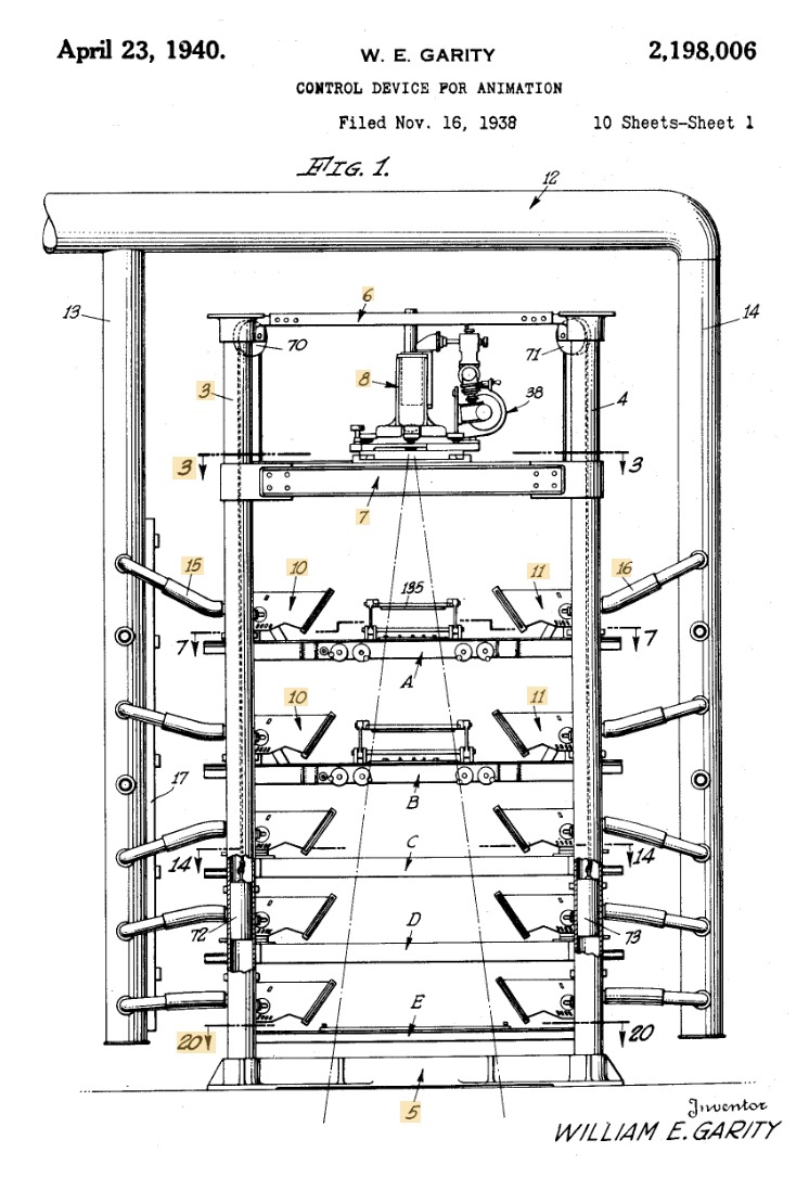
Animators for these cartoons used a device called a multiplane camera, which worked as follows. A camera looked at a stack of glass planes. On each plane, the animators would draw a different layer of the scene. For example, on the back plane would be the sky, then there would be mountains on the next plane, then trees, and then the foreground characters. During filming the planes could be shifted back and forth to create parallax where the foreground planes move by more quickly than the planes further back.
This device works because it is a rough approximation to the actual 3D structure of the world. In computer vision, layer-based representations like this have been popular as a way of capturing some aspects of depth without the expense of modeling a fully 3D world; sometimes layers and other related pseudo-3D representations are called 2.5D representations.
Layers are not just an approximation to true depth, but also capture geometric structure that is not well-represented by depth. Consider a pile of papers on your desk. The depth difference between one page and the next might only be a millimeter—too small to show up on standard depth sensing cameras. But the layer structure is obvious. Look back at Figure 31.2: the depth order is obvious even though you might have no idea how far apart these objects are in metric space. Layers capture ordinal structure and often this is the structure we care about; for example, if we want to pick up a piece of paper in our pile, the main thing that matters is if it is on top.
31.6 Emergent Groups
It may seem like some of the topics in this chapter are out of fashion in modern computer vision. Edge detection and bottom-up segmentation are not the workhorses they once were. But this doesn’t mean that perceptual organization is absent from current systems. These systems still see the world in terms of objects, contours, layers, and so forth, but those structures are emergent in their hidden layers rather than made explicit by human design. For example, in Figure 30.9 we observed object detectors inside a neural net trained to do colorization.
31.7 Concluding Remarks
Perceptual organization aims to represent visual content in terms of modular and disentangled elements that make subsequent processing easier. In this way, perceptual organization shares the same goal as visual representation learning, although the former deals more with discrete structures whereas the latter has focused mostly on continuous representations. These two fields evolved somewhat separately, with perceptual organization having its roots in psychology and representation learning coming more from machine learning, but these days the end result is converging in the form of vision systems that see the world in terms of objects, parts, relationships, layers, and many other useful structures.