25 Recurrent Neural Nets
25.1 Introduction
RNNs are a neural net architecture for modeling sequences—they perform sequential computation (rather than parallel computation).
So far we have seen feedforward neural net architectures. These architectures can be represented by directed acyclical computation graphs. (RNNs), are neural nets with feedback connections.
A feedback connection defines a recurrence in the computational graph.
Their computation graphs have cycles. That means that the outputs of one layer can send a message back to earlier in the computational pipeline. To make this well-defined, RNNs introduce the notion of timestep. One timestep of running an RNN corresponds to one functional call to each layer (or computation node) in the RNN, mapping that layer’s inputs to its outputs.
RNNs are all about adaptation. They solve the following problem: What if we want our computations in the past to influence our computations in the future? If we have a stream of data, a feedforward net has no way to adapting its behavior based on what outputs it previously produced.
To motivate RNNs, we will first consider a deficiency of convolutional neural nets (CNNs). Consider that we are processing a temporal signal with a CNN, like so:
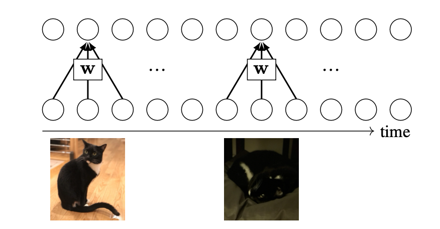
The filter \(\mathbf{w}\) slides over the input signal and produces outputs. In this example, imagine the input is a video of your cat, named Mo. The output produced for the first set of frames is entirely independent from the output produced for a later frame, as long as the receptive fields do not overlap. This independence can cause problems. For instance, maybe it got dark outside as the video progressed, and a clear image of Mo became hard to discern as the light dimmed. Then the convolutional response, and the net’s prediction, for later in the video cannot reference the earlier clear image, and will be limited to making the best inference it can from the dim image.
Wouldn’t it be nice if we could inform the CNN’s later predictions that earlier in the day we had a brighter view and this was clearly Mo? With a CNN, the only way to do this is to increase the size of the convolutional filters so that the receptive fields can see sufficiently far back in time. But what if we last saw Mo a year ago? It would be infeasible to extend our receptive fields a year back. How can we humans solve this problem and recognize Mo after a year of not seeing her?
The answer is memory. The recurrent feedback loops in an RNN are a kind of memory. They propagate information from timestep \(t\) to timestep \(t+1\). In other words, they remember information about timestep \(t\) when processing new information at timestep \(t+1\). Thus, by induction, an RNN can potentially remember information over arbitrarily long time intervals. In fact, RNNs are Turing complete: you can think of them as a little computer. They can do anything a computer can do.
Here’s how RNNs arrange their connections to perform this propagation:
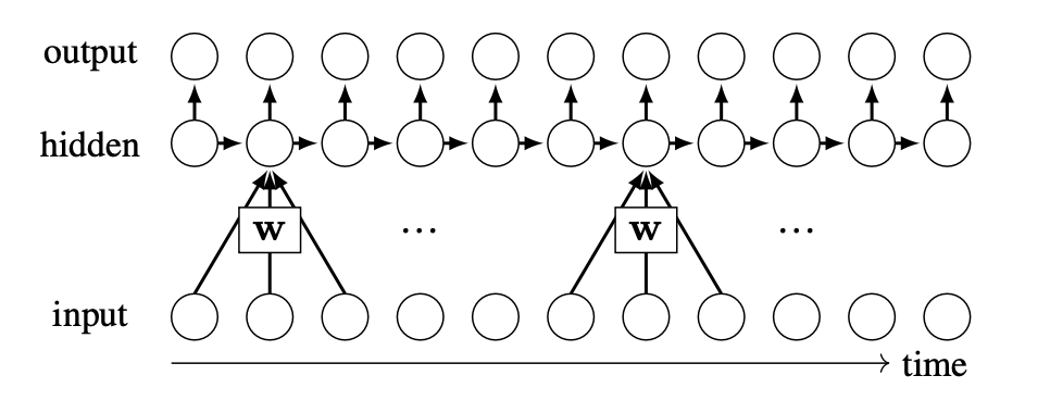
The key idea of an RNN is that there are lateral connections, between hidden units, through time. The inputs, outputs, and hidden units may be multidimensional tensors; to denote this we will use  , as
, as  was reserved for denoting a single (scalar) neuron.
Here is a simple 1-layer RNN:
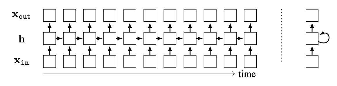
To the left, is the unrolled computation graph. To the right, is the computation graph rolled up, with a feedback connection. Typically we will work with unrolled graphs because they are directed acyclic graphs (DAGs), and therefore all the tools we have developed for DAGs, including backpropagation, will extend naturally to them. However, note that RNNs can run for unbounded time, and process signals that have unbounded temporal extent, while a DAG can only represent a finite graph. The DAG depicted above is therefore a truncated version of the RNN’s theoretical computation graph.
25.2 Recurrent Layer
A is defined by the following equations: \[\begin{aligned} \mathbf{h}_t &= f(\mathbf{h}_{t-1}, \mathbf{x}_{\texttt{in}}[t]) &\triangleleft \quad\quad \text{update state based on input and previous state}\\ \mathbf{x}_{\texttt{out}}[t]&= g(\mathbf{h}_t) &\triangleleft \quad\quad \text{produce output based on state} \end{aligned}\]
This is a layer that includes a state variable, \(\mathbf{h}\). The operation of the layer depends on its state. The layer also updates its state every time it is called, therefore the state is a kind of memory.
The idea of a time in an RNN does not necessarily mean time as it is measured on a clock. Time just refers to sequential computation; the timestep \(t\) is an index into the sequence. The sequential computation could progress over a spatial dimension (processing an image pixel by pixel) or over the temporal dimension (processing a video frame by frame), or even over more abstracted computational modules.
The \(f\) and \(g\) can be arbitrary functions, and we can imagine a wide variety of recurrent layers defined by different choices for the form of \(f\) and \(g\).
One common kind of recurrent layer is the (SRN), which was defined by Elman in “Finding Structure in Time” [1]. For this layer, \(f\) is a linear layer followed by a pointwise nonlinearity, and \(g\) is another linear layer. The full computation is defined by the following equations: \[\begin{aligned} \mathbf{h}_t &= \sigma_1(\mathbf{W}\mathbf{h}_{t-1} + \mathbf{U}\mathbf{x}_{\texttt{in}}[t]+ \mathbf{b})\\ \mathbf{x}_{\texttt{out}}[t]&= \sigma_2(\mathbf{V}\mathbf{h}_t + \mathbf{c}) \end{aligned}\] where \(\sigma_1\) and \(\sigma_2\) are pointwise nonlinearities. In SRNs, tanh is the common choice for the nonlinearity, but relus and other choices may also be used.
25.3 Backpropagation through Time
Backpropagation is only defined for DAGs and RNNs are not DAGs. To apply backpropagation to RNNs, we unroll the net for \(T\) timesteps, which creates a DAG representation of the truncated RNN, and then do backpropagation through that DAG. This is known as (BPTT).
This approach yields exact gradients of the loss with respect to the parameters when \(T\) is equal to the total number of timesteps the RNN was run for. Otherwise, BPTT is an approximation that truncates the true computation graph. Essentially, BPTT ignores any dependencies in the computation graph greater than length \(T\).
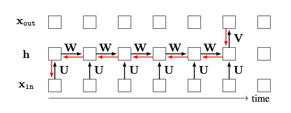
As an example of BPTT, suppose we want to compute the gradient of an output neuron at timestep five with respect to an input at timestep zero, that is, \(\frac{\partial \mathbf{x}_{\texttt{out}}[5]}{\partial \mathbf{x}_{\texttt{in}}[0]}\). The forward pass (black arrows) and backward pass (red arrows) are shown in Figure 25.4, where we have only drawn arrows for the subpart of the computation graph that is relevant to the calculation of this particular gradient.
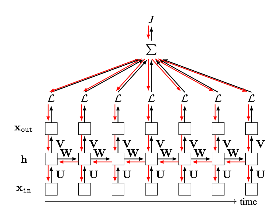
What about the gradient of the total cost with respect to the parameters, \(\frac{\partial J}{\partial [\mathbf{W}, \mathbf{U}, \mathbf{V}]}\)? Suppose the RNN is being applied to a video and predicts a class label for every frame of the video. Then \(\mathbf{x}_{\texttt{out}}\) is a prediction for each frame and a loss can be applied to each \(\mathbf{x}_{\texttt{out}}[t]\). The total cost is simply the summation of the losses at each timestep: \[\begin{aligned} \frac{\partial J}{\partial [\mathbf{W}, \mathbf{U}, \mathbf{V}]} = \sum_{t=0}^T \frac{\partial \mathcal{L}(\mathbf{x}_{\texttt{out}}[t], \mathbf{y}_t)}{\partial [\mathbf{W}, \mathbf{U}, \mathbf{V}]} \end{aligned}\] The graph for backpropagation, shown in Figure 25.5, has a branching structure, which we saw how to deal with in Chapter 14: gradients (red arrows) summate wherever the forward pass (black arrows) branches.
25.3.1 The Problem of Exploding and Vanishing Gradients
Notice that the we can get very large computation graphs when we run an RNN for many timesteps. The gradient computation involves a series of matrix multiplies that is \(\mathcal{O}(T)\) in length. For example, to compute our gradient \(\frac{\partial \mathbf{x}_{\texttt{out}}[5]}{\partial \mathbf{x}_{\texttt{in}}[0]}\) in the example above involves the following product:
\[\begin{aligned} \frac{\partial \mathbf{x}_{\texttt{out}}[t]}{\partial \mathbf{x}_{\texttt{in}}[0]} = \frac{\partial \mathbf{x}_{\texttt{out}}[t]}{\partial \mathbf{h}_T} \frac{\partial \mathbf{h}_T}{\partial \mathbf{h}_{T-1}} \cdots \frac{\partial \mathbf{h}_1}{\partial \mathbf{h}_0} \frac{\partial \mathbf{h}_0}{\partial \mathbf{x}_{\texttt{in}}[0]} \end{aligned}\]
Suppose we use an RNN with relu nonlinearities. Then each term \(\frac{\partial \mathbf{h}_t}{\partial \mathbf{h}_{t-1}}\) equals \(\mathbf{R}\mathbf{W}\), where \(\mathbf{R}\) is a diagonal matrix with zeros or ones on the \(i\)-th diagonal element depending on whether the \(i\)-th neuron is above or below zero at the current operating point. This gives a product \(\mathbf{R}_T\mathbf{W}\cdots\mathbf{R}_1\mathbf{W}\). In a worst-case scenario (for numerics), suppose all the \(\texttt{relu}\) are active; then we have a product of \(T\) matrices \(\mathbf{W}\), which means the gradient is \(\mathbf{W}^T\) (\(T\) is an exponent here, not a transpose). If values in \(\mathbf{W}\) are large, the gradient will explode. If they are small, the gradient will vanish—basically, this system is not numerically well-behaved. One solution to this problem is to use RNN units that have better numerics, an example of which we will give in Section 25.5 subsequently.
25.4 Stacking Recurrent Layers
A deep RNN can be constructed by stacking recurrent layers. Here is an example:
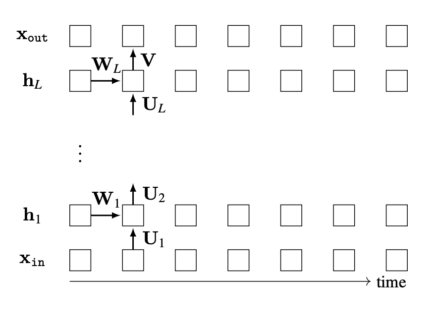
To emphasize that the parameters are shared, we only show them once.
Here is code for a two-layer version of this RNN:
# d_in, d_hid, d_out: input, hidden, and output dimensionalities
# x : input data sequence
# h_init: initial conditions of hidden state
# T: number of timesteps to run for

# first define parameterized layers
U1 = nn.fc(dim_in=d_in, dim_out=d_hid, bias=False)
U2 = nn.fc(dim_in=d_hid, dim_out=d_hid, bias=False)
W1 = nn.fc(dim_in=d_hid, dim_out=d_hid)
W2 = nn.fc(dim_in=d_hid, dim_out=d_hid)
V = nn.fc(dim_in=d_hid, dim_out=d_out)

# then run data through network
h1, h2 = h_init
for t in range(T):
    h1[t] = nn.tanh(W1(h1[t-1])+U1(x[t]))
    h2[t] = nn.tanh(W2(h2[t-1])+U2(h1[t]))
    x_out[t] = V(h2[t])
We set the bias to be “False” for \(\mathbf{U}_1\) and \(\mathbf{U}_2\) since the recurrent layer already gets a bias term from \(\mathbf{W}_1\) and \(\mathbf{W}_2\).
25.5 Long Short-Term Memory
(LSTMs) are a special kind of recurrent module, that is designed to avoid the vanishing and exploding gradients problem described in Section 25.3.1 [2].
The presentation of LSTMs in this section draws inspiration from a great blog post by Chris Olah .
An LSTM is like a little memory controller. It has a cell state, \(\mathbf{c}\), which is a vector it can read from and write to. The cell state can record memories and retrieve them as needed. The cell state plays a similar role as the hidden state, \(\mathbf{h}\), from regular RNNs—both record memories—but the cell state is built to store persistent memories that can last a long time (hence the name long short-term memory). We will see how next.
Like a normal recurrent layer, an LSTM takes as input a hidden state \(\mathbf{h}_{t-1}\) and an observation \(\mathbf{x}_{\texttt{in}}[t]\) and produces as output an updated hidden state \(\mathbf{h}_t\). Internally, the LSTM uses its cell state to decide how to update \(\mathbf{h}_{t-1}\).
First, the cell state is updated based on the incoming signals, \(\mathbf{h}_{t-1}\) and \(\mathbf{x}_{\texttt{in}}[t]\). Then the cell state is used to determine the hidden state \(\mathbf{h}_{t}\) to output. Different subcomponents of the LSTM layer decide what to delete from the cell state, what to write to the cell state, and what to read off the cell state.
One component picks the indices of the cell state to delete: \[\begin{aligned} \mathbf{f}_t &= \sigma(\mathbf{W}_f\mathbf{h}_{t-1} + \mathbf{U}_f\mathbf{x}_{\texttt{in}}[t] + \mathbf{b}_f) &\triangleleft \quad\quad\text{decide which indices to forget} \end{aligned}\] where \(\mathbf{f}_t\) is a vector of length equal to the length of the cell state \(\mathbf{c}_t\), and \(\sigma\) is the sigmoid function that outputs values in the range \([0,1]\). The idea is that most values in \(\mathbf{f}_t\) will be near either \(1\) (remember) or 0 (forget). Later \(\mathbf{f}_t\) will be pointwise multiplied by the cell state to forget the values where \(\mathbf{f}_t\) is zero.
Another component chooses what values to write to the cell state, and where to write them: \[\begin{aligned} \mathbf{i}_t &= \sigma(\mathbf{W}_i\mathbf{h}_{t-1} + \mathbf{U}_i\mathbf{x}_{\texttt{in}}[t] + \mathbf{b}_i) &\triangleleft \quad\quad\text{which indices to write to}\\ \tilde{\mathbf{c}}_t &= \texttt{tanh}(\mathbf{W}_C\mathbf{h}_{t-1} + \mathbf{U}_c\mathbf{x}_{\texttt{in}}[t] + \mathbf{b}_c) &\triangleleft \quad\quad\text{what to write to those indices} \end{aligned}\] where \(\mathbf{i}_t\) is similar to \(\mathbf{f}_t\) (it’s a vector whose values that are nearly 0 or 1 of length equal to the length of the cell state) and it determines which indices of \(\tilde{\mathbf{c}}_t\) will be written to the cell state. Next we use these vectors to actually update the cell state: \[\begin{aligned} \mathbf{c}_t &= \mathbf{f}_t \odot \mathbf{c}_{t-1} + \mathbf{i}_t \odot \tilde{\mathbf{c}}_{t} &\triangleleft \quad\quad\text{update the cell state} \end{aligned}\]
Finally, given the updated cell state, we read from it and use the values to determine the hidden state to output: \[\begin{aligned} \mathbf{o}_t &= \sigma(\mathbf{W}_o\mathbf{h}_{t-1} + \mathbf{U}_o\mathbf{x}_{\texttt{in}}[t] + \mathbf{b}_o) &\triangleleft \quad\quad\text{which indices of cell state to use}\\ \mathbf{h}_t &= \mathbf{o}_t \odot \texttt{tanh}(\mathbf{c}_t) &\triangleleft \quad\quad\text{use these to determine next hidden state} \end{aligned}\] The basic idea is it should be easy, by default, not to forget. The cell state controls what is remembered. It gets modulated, but \(\mathbf{f}_t\) can learn to be all ones so that information propagates forward through an identity connection from the previous cell state to the subsequent cell state. This idea is similar to the idea of skip connections and residual connections in U-Nets and ResNets Chapter 24.
25.6 Concluding Remarks
Recurrent connections give neural nets the ability to maintain a persistent state representation, which can be propagated forward in time or can be updated in the face of incoming experience. The same idea has been proposed in multiple fields: in control theory it is the basic distinction between open-loop and closed-loop control. Closed-loop control allows the controller to change its behavior based on feedback from the consequences of its previous decisions; similarly, recurrent connections allow a neural net to change its behavior based on feedback, but the feedback is from downstream processing all within the same neural net. Feedback is a fundamental mechanism for making systems that are adaptive. These systems can become more competent the longer you run them.