23 Image Pyramids
23.1 Introduction
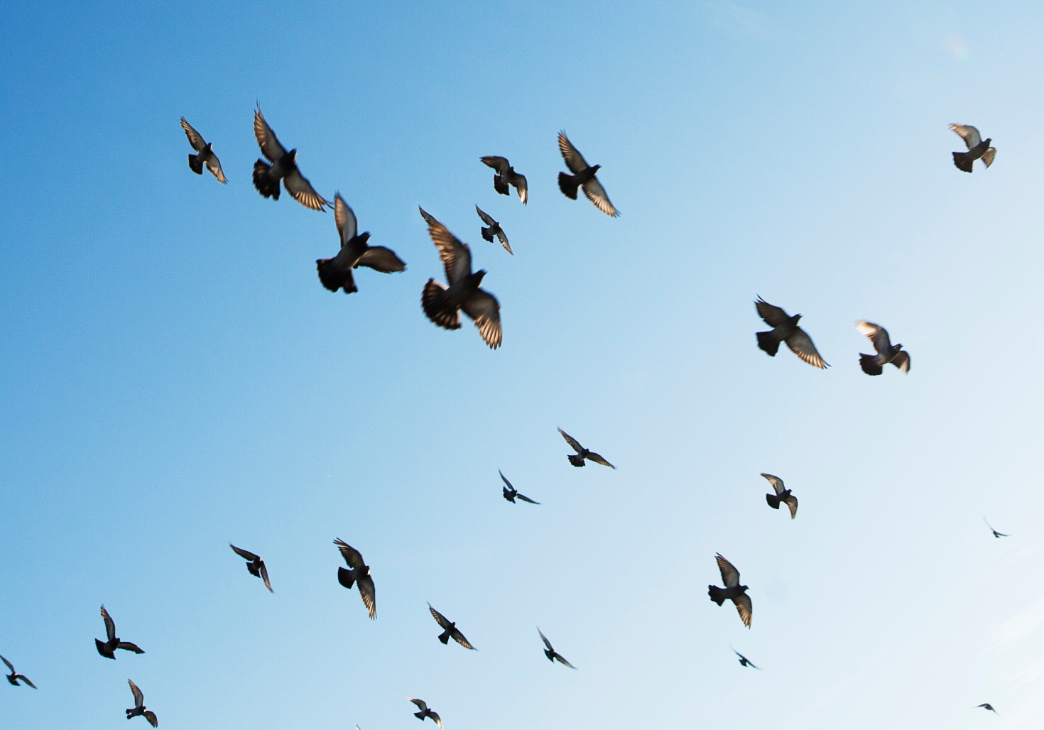
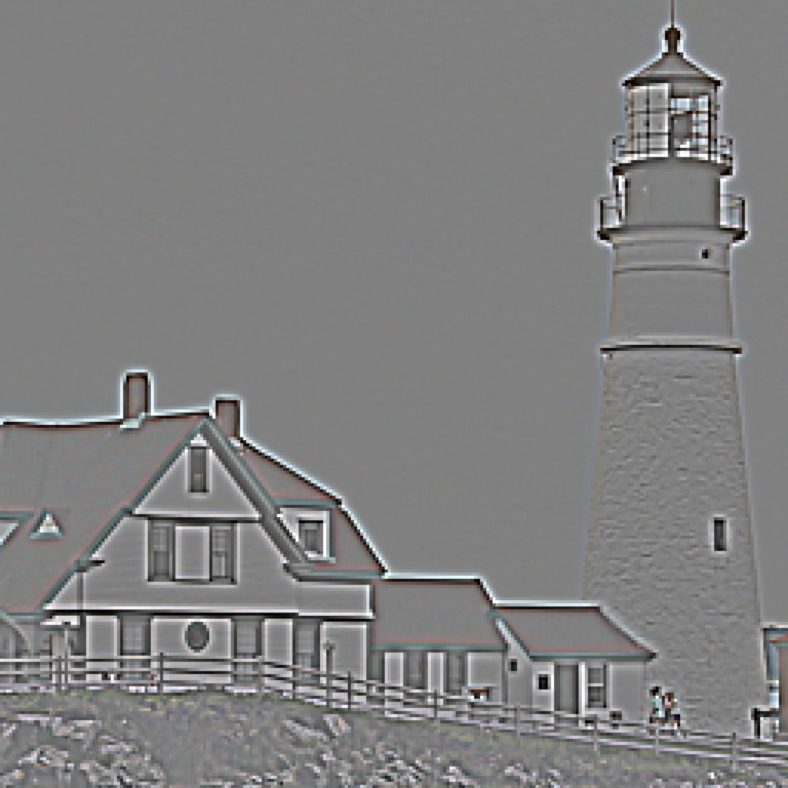
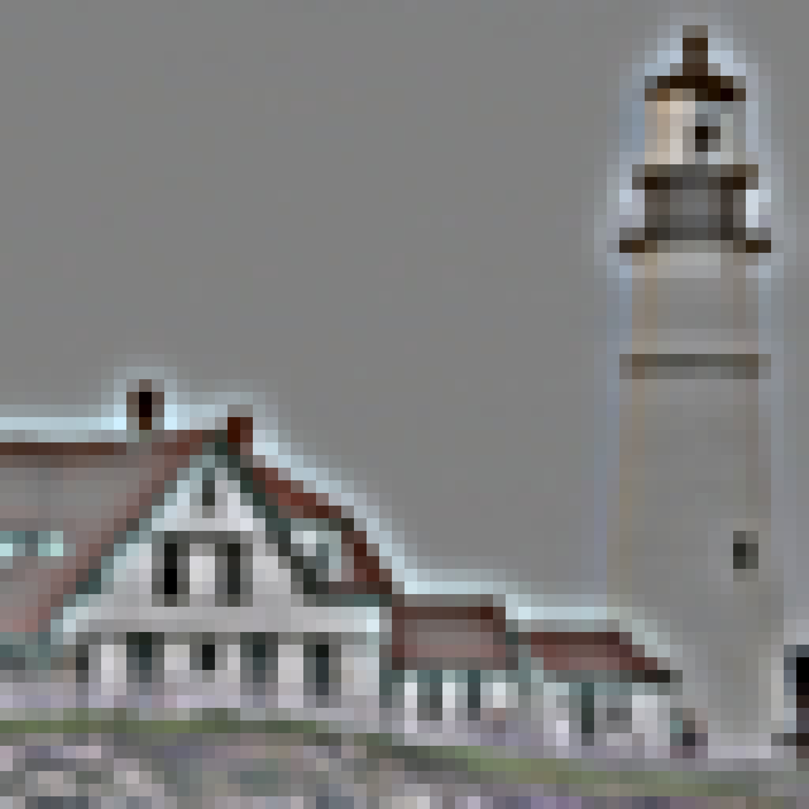
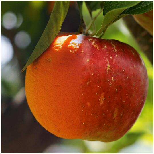
In Chapter 15 we motivated translation invariant linear filters as a way of accounting for the fact that objects in images might appear at any location. Therefore, a reasonable way of processing an image is by manipulating pixel neighborhoods in the same way independently on the image location. In addition to translation invariance, scale invariance is another fundamental property of images. Due to perspective projection, objects at different distances will appear with different sizes as shown in Figure 23.1. Therefore, if we want to locate all the bird instances in this image, we will have to apply an operator that is invariant in translation and in scale. Image pyramids provide an efficient representation for space-scale invariant processing.
23.2 Image Pyramids and Multiscale Image Analysis
Image information occurs over many different spatial scales. Image pyramids (i.e., multiresolution representations for images) are a useful data structure for analyzing and manipulating images over a range of spatial scales. Here we’ll discuss three different ones, in a progression of complexity. The first is a Gaussian pyramid, which creates versions of the input image at multiple resolutions. This is useful for analysis across different spatial scales, but doesn’t separate the image into different frequency bands. The Laplacian pyramid provides that extra level of analysis, breaking the image into different isotropic spatial frequency bands. The steerable pyramid provides a clean separation of the image into different scales and orientations. There are various other differences between these pyramids, which we’ll describe below.
As a motivating example, let’s assume we want to detect the birds from Figure 23.1. If we have a template of a bird, normalized correlation will be able to detect only the birds that have a similar image size than the template. To introduce scale invariance, one possible solution is to change the size of the template to cover a wide range of possible sizes and apply them to the image. Then, the ensemble of templates will be able to detect birds of different sizes. The disadvantage of this approach is that it will be computationally expensive as detecting large birds will require computing convolutions with big kernels, which is very slow. Another alternative is to change the image size as shown in Figure 23.2, resulting in a multiscale image pyramid.
In this example, the original image has a resolution of 848 \(\times\) 643 pixels. Each image in the pyramid is obtained by scaling down the image from the previous level by reducing the number of pixels by a factor of \(25\) percent (that is, each image in the pyramid has 3/4 of the size of the precedent image).
Downsampling is discussed in detail in Chapter 21.
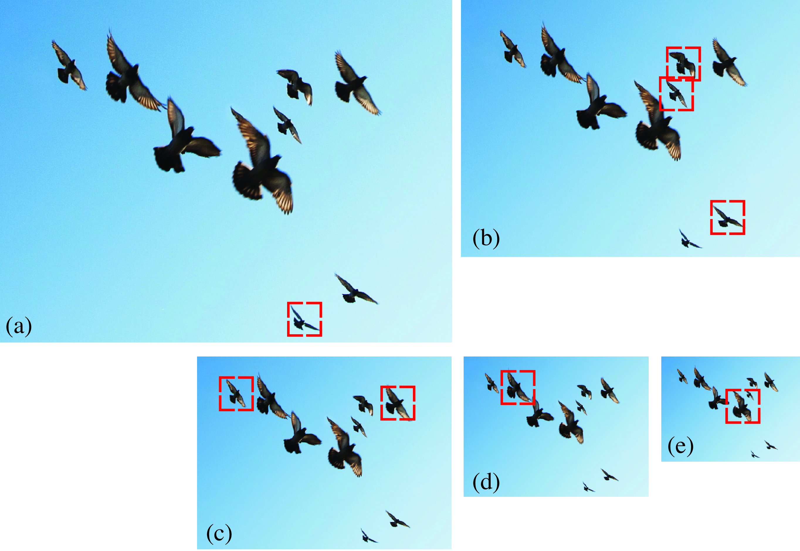
Now we can use the pyramid to detect birds at different sizes using a single template. The red box in the figure denotes the size of the template used. The figure shows how birds of different sizes become detectable at, at least, one of the levels of the pyramid. This method will be more efficient as the template can be kept small and the convolutions will remain computationally efficient.
Mutiscale image processing and image pyramids have many applications beyond scale invariant object detection. In this chapter we will describe some important image pyramids and their applications.
23.3 Linear Image Transforms
Let’s first look at some general properties of linear image transforms. For an input image \(\boldsymbol\ell\) with \(N\) pixels, a linear transform is: \[\mathbf{r} = \mathbf{P}^\mathsf{T}\boldsymbol\ell\] where \(\mathbf{r}\) is a vector of dimensionality \(M\), and \(\mathbf{P}\) is a matrix of size \(N \times M\). The columns of \(\mathbf{P} = \left[\mathbf{P}_0, \mathbf{P}_1, ...,\mathbf{P}_{M-1}\right]\) are the projection vectors. The vector \(\mathbf{r}\) contains the transform coefficients: \(\mathbf{r}_i = \mathbf{P}_i^\mathsf{T}\boldsymbol\ell\). The vector \(\mathbf{r}\) corresponds to a different representation of the image \(\boldsymbol\ell\) than the original pixel space.
We are interested in transforms that are invertible, so that we can recover the input \(\boldsymbol\ell\) from the projection coefficients \(\mathbf{r}\): \[\boldsymbol\ell= \mathbf{Q} \mathbf{r} = \sum_{i=0}^{M-1} \mathbf{r}_i \mathbf{Q}_i\] The columns of \(\mathbf{Q}= \left[\mathbf{Q}_0, \mathbf{Q}_1, ...,\mathbf{Q}_{M-1}\right]\) are the basis vectors. The input signal \(\boldsymbol\ell\) can be reconstructed as a linear combination of the basis vectors \(\mathbf{Q}_i\) weighted by the representation coefficients \(\mathbf{r}_i\).
The transform \(\mathbf{P}\) is said to be critically sampled when \(M=N\). The transform is oversampled when \(M > N\), and undersampled when \(M < N\). The transform \(\mathbf{P}\) is complete, that is, encoding all image structure, if it is invertible. If critically sampled (i.e., \(M=N\)) and the transform is complete, then \(\mathbf{Q} = (\mathbf{P}^\mathsf{T})^{-1}\). If it is overcomplete (oversampled and complete), then the inverse can be obtained using the pseudoinverse \(\mathbf{Q}=(\mathbf{P} \mathbf{P}^\mathsf{T})^{-1}\mathbf{P}\).
An important special case is when the transform is self-inverting, then \(\mathbf{P} \mathbf{P}^{\mathsf{T}} = \mathbf{I}\). The values of \(\mathbf{P}\) can be real or complex (like in the Fourier transform). For complex transforms, we should replace the \(\mathbf{P}^\mathsf{T}\) by \(\mathbf{P}^{*\mathsf{T}}\) (i.e., complex conjugate transpose).
The quadrature mirror filter (QMF) transform is an example of self-inverting transform [1]. For 1D signals of length 4, the QMF transform can be written as: \[ \mathbf{P}=\frac{1}{\sqrt{2}} \begin{bmatrix} 1 ~& 1 ~& 0 ~& 0 \\ 1 ~& -1 ~& 0 ~& 0 \\ 0 ~& 0 ~& 1 ~& 1 \\ 0 ~& 0 ~& 1 ~& -1 \end{bmatrix} \] This is equivalent to the convolution of the input signal with two orthogonal kernels, \([1,1]\) and \([1,-1]\), with a stride of 2.
This transform also has a multiscale version that is also self-inverting: \[ \mathbf{P}= \begin{bmatrix} \frac{1}{\sqrt{2}} & -\frac{1}{\sqrt{2}} & 0 & 0 \\[5pt] 0 & 0 & \frac{1}{\sqrt{2}} & -\frac{1}{\sqrt{2}} \\[5pt] \frac{1}{2} & \frac{1}{2} & \frac{1}{2} & \frac{1}{2} \\[5pt] \frac{1}{2} & \frac{1}{2} & -\frac{1}{2} & -\frac{1}{2} \end{bmatrix} \] You can check that in both cases \(\mathbf{Q} = \left( \mathbf{P^\mathsf{T}} \right) ^{-1} = \mathbf{P^\mathsf{T}}\). These transforms can be extended to 2D.
23.4 Gaussian Pyramid
We’d like to make a recursive algorithm for creating a multiresolution version of an image. A Gaussian filter is a natural one to use to blur out an image, since the multiple successive application of a Gaussian filter is equivalent to application of a single, wider Gaussian filter.
Here’s an elegant, efficient algorithm for making a resolution–reduced version of an input image. It involves two steps: convolving the image with a low-pass filter (e.g., using the fourth binomial filter \(\mathbf{b}_4 = [1, 4, 6, 4, 1]\) / 16, normalized to sum to 1, separably in each dimension), and then subsampling by a factor of 2 the result. Each level is obtained by filtering the previous level with the fourth binomial filter with a stride of 2 (on each dimension). Applied recursively, this algorithm generates a sequence of images, subsequent ones being smaller, lower resolution versions of the earlier ones in the processing.
Figure 23.3 shows the Gaussian pyramid of an image with six levels. Each level has half the resolution of the previous level.


To make the filters more intuitive, it is useful to write the two steps in matrix form. The following matrix shows the recursive construction of level \(k+1\) of the Gaussian pyramid for a one-dimensional (1D) image: \[\mathbf{g}_{k+1} = \mathbf{D}_k \mathbf{B}_k \mathbf{g}_k = \mathbf{G}_k \mathbf{g}_k\] where \(\mathbf{D}_k\) is the downsampling operator, \(\mathbf{B}_k\) is the convolution with the fourth binomial filter, and \(\mathbf{G}_k = \mathbf{D}_k \mathbf{B}_k\) is the blur-and-downsample operator for level \(k\).
One block of the Gaussian pyramid computation. 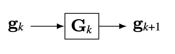
We call the sequence of images \(\mathbf{g}_0, \mathbf{g}_1, . . ., \mathbf{g}_N\) as the Gaussian pyramid. The first level of the Gaussian pyramid is the input image: \(\mathbf{g}_0=\boldsymbol\ell\).
It is useful to check a concrete example. If \(\mathbf{x}\) is a 1D signal of length 8, and if we assume zero boundary conditions, the matrices for computing \(\mathbf{g}_1\) are: \[\mathbf{G}_0 = \mathbf{D}_0 \mathbf{B}_0 = \begin{bmatrix} 1 ~& 0 ~& 0 ~& 0 ~& 0 ~& 0 ~& 0 ~& 0 \\ 0 ~& 0 ~& 1 ~& 0 ~& 0 ~& 0 ~& 0 ~& 0 \\ 0 ~& 0 ~& 0 ~& 0 ~& 1 ~& 0 ~& 0 ~& 0 \\ 0 ~& 0 ~& 0 ~& 0 ~& 0 ~& 0 ~& 1 ~& 0 \end{bmatrix} \frac{1}{16} \begin{bmatrix} 6 ~& 4 ~& 1 ~& 0 ~& 0 ~& 0 ~& 0 ~& 0 \\ 4 ~& 6 ~& 4 ~& 1 ~& 0 ~& 0 ~& 0 ~& 0 \\ 1 ~& 4 ~& 6 ~& 4 ~& 1 ~& 0 ~& 0 ~& 0 \\ 0 ~& 1 ~& 4 ~& 6 ~& 4 ~& 1 ~& 0 ~& 0 \\ 0 ~& 0 ~& 1 ~& 4 ~& 6 ~& 4 ~& 1 ~& 0 \\ 0 ~& 0 ~& 0 ~& 1 ~& 4 ~& 6 ~& 4 ~& 1 \\ 0 ~& 0 ~& 0 ~& 0 ~& 1 ~& 4 ~& 6 ~& 4 \\ 0 ~& 0 ~& 0 ~& 0 ~& 0 ~& 1 ~& 4 ~& 6 \end{bmatrix}\] Multiplying the two matrices: \[\mathbf{g}_{1} = \mathbf{G}_0 \boldsymbol\ell= \frac{1}{16} \begin{bmatrix} 6 ~& 4 ~& 1 ~& 0 ~& 0 ~& 0 ~& 0 ~& 0 \\ 1 ~& 4 ~& 6 ~& 4 ~& 1 ~& 0 ~& 0 ~& 0 \\ 0 ~& 0 ~& 1 ~& 4 ~& 6 ~& 4 ~& 1 ~& 0 \\ 0 ~& 0 ~& 0 ~& 0 ~& 1 ~& 4 ~& 6 ~& 4 \end{bmatrix} \boldsymbol\ell\] the first level of the Gaussian pyramid is a signal \(\mathbf{g}_1\) with length 4. Applying the recursion we can write the output of each level as a function of the input \(\boldsymbol\ell\): \(\mathbf{g}_{2} = \mathbf{G}_1 \mathbf{G}_0 \boldsymbol\ell\), \(\mathbf{g}_{3} = \mathbf{G}_2 \mathbf{G}_1 \mathbf{G}_0 \boldsymbol\ell\), and so on.
23.5 Laplacian Pyramid
In the Gaussian pyramid, each level losses some of the fine image details available in the previous level. The Laplacian pyramid [2] is simple: it represents, at each level, what is present in a Gaussian pyramid image of one level, but not present at the level below it. We calculate that by expanding the lower-resolution Gaussian pyramid image to the same pixel resolution as the neighboring higher-resolution Gaussian pyramid image, then subtracting the two. This calculation is made in a recursive, telescoping fashion.
Let’s look at the steps for calculating a Laplacian pyramid. What we want is to compute the difference between \(\mathbf{g}_k\) and \(\mathbf{g}_{k+1}\). To do this first we need to upsample the image \(\mathbf{g}_{k+1}\) so that it has the same size as \(\mathbf{g}_k\). Let \(\mathbf{F}_k = \mathbf{B}_k \mathbf{U}_k\) be the upsample-and-blur operator for pyramid level \(k\). The operator \(\mathbf{F}_k\) applies first the upsampling operator \(\mathbf{U}_k\), that inserts zeros between samples, followed by blurring by the same filter \(\mathbf{B}_k\) than the one we used for the Gaussian pyramid. The Laplacian pyramid coefficients, \(\mathbf{l}_k\), at pyramid level \(k\), are: \[\mathbf{l}_{k} = \mathbf{g}_k - \mathbf{F}_k \mathbf{g}_{k+1} = (\mathbf{I}_k - \mathbf{F}_k \mathbf{G}_k) \mathbf{g}_{k} = \mathbf{L}_k \mathbf{g}_{k} \tag{23.1}\]
One block of the Laplacian pyramid computation.
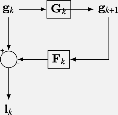
Figure 23.4 shows the resulting Laplacian pyramid for an image. To compute a Laplacian pyramid with \(N\) levels, we need to first compute the Gaussian pyramid of the input image with \(N+1\) levels. The last level of this pyramid is the smallest level of the Gaussian pyramid used to compute the Laplacian pyramid and is called the low-pass residual.

The Laplacian pyramid is built for each color channel independently.
Let’s write down the matrices in Equation 23.1 for a 1D input \(\boldsymbol\ell\) of length 8, and assuming zero boundary conditions. The operators to compute the first level (\(k=0\)) of the Laplacian pyramid are: \[\mathbf{F}_0 = 2 \mathbf{B}_0 \mathbf{U}_0 = \frac{1}{8} \begin{bmatrix} 6 ~& 4 ~& 1 ~& 0 ~& 0 ~& 0 ~& 0 ~& 0 \\ 4 ~& 6 ~& 4 ~& 1 ~& 0 ~& 0 ~& 0 ~& 0 \\ 1 ~& 4 ~& 6 ~& 4 ~& 1 ~& 0 ~& 0 ~& 0 \\ 0 ~& 1 ~& 4 ~& 6 ~& 4 ~& 1 ~& 0 ~& 0 \\ 0 ~& 0 ~& 1 ~& 4 ~& 6 ~& 4 ~& 1 ~& 0 \\ 0 ~& 0 ~& 0 ~& 1 ~& 4 ~& 6 ~& 4 ~& 1 \\ 0 ~& 0 ~& 0 ~& 0 ~& 1 ~& 4 ~& 6 ~& 4 \\ 0 ~& 0 ~& 0 ~& 0 ~& 0 ~& 1 ~& 4 ~& 6 \end{bmatrix} \begin{bmatrix} 1 ~& 0 ~& 0 ~& 0\\ 0 ~& 0 ~& 0 ~& 0\\ 0 ~& 1 ~& 0 ~& 0\\ 0 ~& 0 ~& 0 ~& 0\\ 0 ~& 0 ~& 1 ~& 0\\ 0 ~& 0 ~& 0 ~& 0\\ 0 ~& 0 ~& 0 ~& 1\\ 0 ~& 0 ~& 0 ~& 0 \end{bmatrix}\] The factor 2 is necessary because inserting zeros decreases the average value of the signal \(\mathbf{g}_{k+1}\) by a factor of 2. Multiplying the two matrices: \[\mathbf{l}_{0} = \mathbf{g}_0 - \mathbf{F}_0 \mathbf{g}_{1} = \mathbf{g}_0 - \frac{1}{8} \begin{bmatrix} 6 ~& 1 ~& 0 ~& 0\\ 4 ~& 4 ~& 0 ~& 0\\ 1 ~& 6 ~& 1 ~& 0\\ 0 ~& 4 ~& 4 ~& 0\\ 0 ~& 1 ~& 6 ~& 1\\ 0 ~& 0 ~& 4 ~& 4\\ 0 ~& 0 ~& 1 ~& 6\\ 0 ~& 0 ~& 0 ~& 4 \end{bmatrix} \mathbf{g}_{1}\] We can also calculate the matrix that should be applied to the input \(\boldsymbol\ell=\mathbf{g_0}\). \[\mathbf{l}_{0} = (\mathbf{I} - \mathbf{F}_0 \mathbf{G}_0) \mathbf{g}_0= \frac{1}{256} \begin{bmatrix} 182 ~& -56 ~& -24 ~& -8 ~& -2 ~& 0 ~& 0 ~& 0\\ -56 ~& 192 ~& -56 ~& -32 ~& -8 ~& 0 ~& 0 ~& 0\\ -24 ~& -56 ~& 180 ~& -56 ~& -24 ~& -8 ~& -2 ~& 0\\ -8 ~&-32 ~& -56 ~& 192 ~& -56 ~& -32 ~& -8 ~& 0\\ -2 ~& -8 ~& -24 ~& -56 ~& 180 ~& -56 ~& -24 ~& -8\\ 0 ~& 0 ~& -8 ~& -32 ~& -56 ~& 192 ~& -56 ~& -32\\ 0 ~& 0 ~& -2 ~& -8 ~& -24 ~& -56 ~& 182 ~& -48\\ 0 ~& 0 ~& 0 ~& 0 ~& -8 ~& -32 ~& -48 ~& 224 \end{bmatrix} \boldsymbol\ell\]
Interestingly, the Laplacian pyramid is an invertible transform, but only if we keep the low-pass residual. We can reconstruct the original image from the Laplacian pyramid. Using the low-pass residual signal associated with the Laplacian pyramid, we can recursively reconstruct the corresponding Gaussian pyramid. Remember that in the Gaussian pyramid level 1 is just the original image itself, so we can use this to reconstruct the original image from the Laplacian pyramid. We can do it recursively applying, from \(k=N-1\) to \(k=0\): \[\mathbf{g}_k = \mathbf{l}_k + \mathbf{F}_k \mathbf{g}_{k+1} \tag{23.2}\]
The diagram in Figure 23.5 shows the Gaussian pyramid, the Laplacian pyramid and the Laplacian inversion for a three-level Laplacian pyramid. The reconstruction uses the Laplacian pyramid \(\mathbf{l}_0,\mathbf{l}_1,...,\mathbf{l}_2\) and the low pass residual \(\mathbf{g}_3\) to recover the input signal \(\boldsymbol\ell=\mathbf{g}_0\).
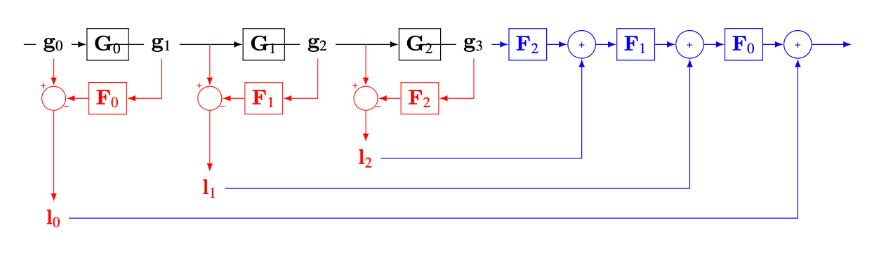
This architecture has two parts: (1) the analysis network (or encoder) that transforms the input image \(\mathbf{x}\) into a representation composed of \(\mathbf{l}_0, \mathbf{l}_1, ...\) and the low pass residual \(\mathbf{x}_n\); and (2) the synthesis network (or decoder) that reconstructs the input from the representation. The Laplacian pyramid is an overcomplete representation (more coefficients than pixels); the dimensionality of the representation is higher than the dimensionality of the input.
Encoder and decoder networks are also common building blocks of deep neural networks. The Laplacian pyramid can be considered as a special type of deep neural net.
Note that the reconstruction property of the Laplacian pyramid does not depend on the filters used for subsampling and upsampling. Even if we used random filters the reconstruction property would still hold.
23.5.1 Image Blending
Image blending (or image compositing) consists in introducing elements of one image inside another. Creating convincing composite images is challenging, as the edge between the two images has to be invisible. One way of formalizing the image-blending operation is by defining a mask, \(\mathbf{m}\), that specifies how the images will be combined. The mask is used to select which pixels come from each of the two images in order to create the composite image. For example, let’s blend two images using the mask as shown in Figure 23.6.
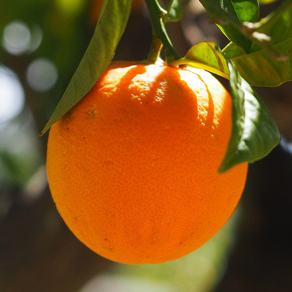
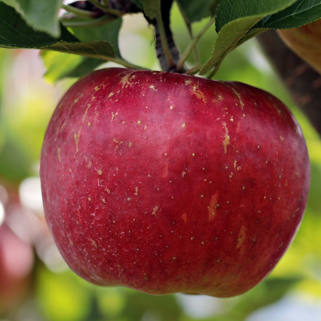

In this example, the mask indicates that the blended image will combine the half-left of the first image with the right-half of the second image. One naive solution to this problem will be to define blending as \(\boldsymbol\ell_{\texttt{out}}= \boldsymbol\ell^A * \mathbf{m} + \boldsymbol\ell^B * (1-\mathbf{m})\), giving as result the image in Figure 23.7.
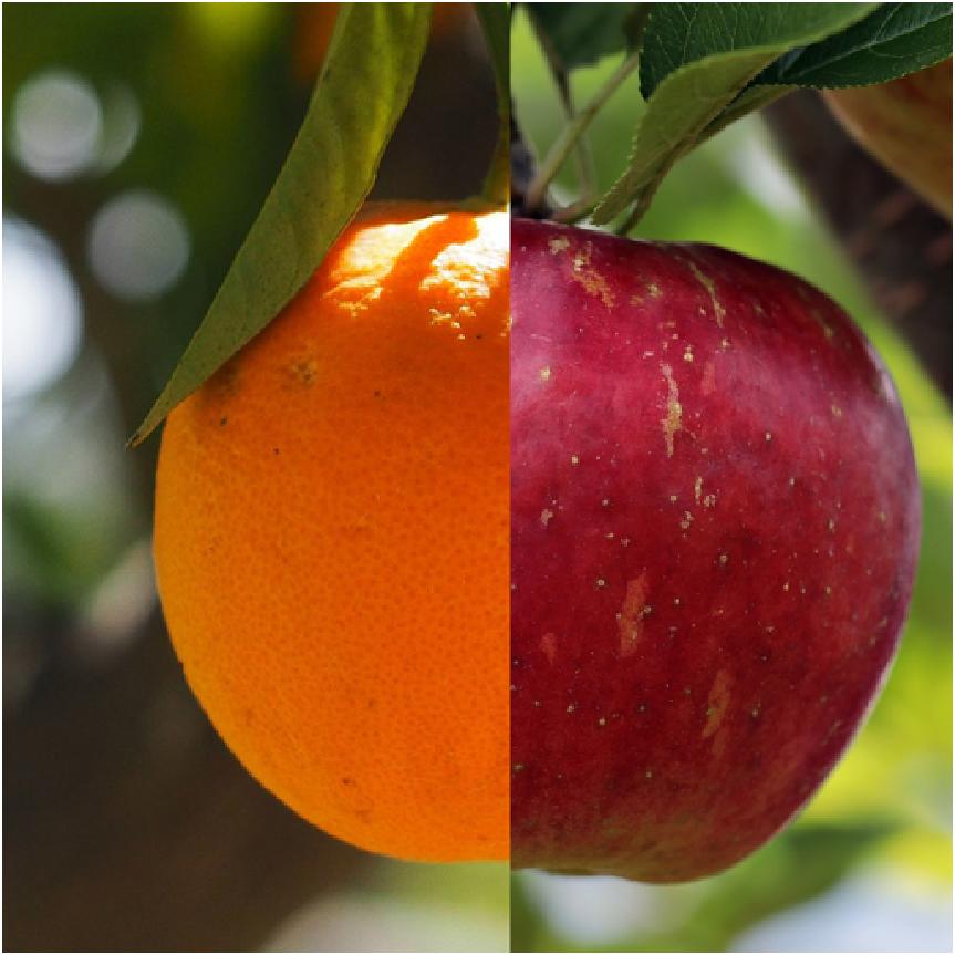
The result in Figure 23.7 is not very pleasing as there is a sharp transition from one image to another (see the straight edge between the two halves of the apple and orange.) We would like to be able to merge both images in a seamless way. In 1983, Burt and Adelson [2] introduced an image blending algorithm using Laplacian pyramid capable of achieve a smooth transition between the two images. This approach remains one of the best solutions to this problem.
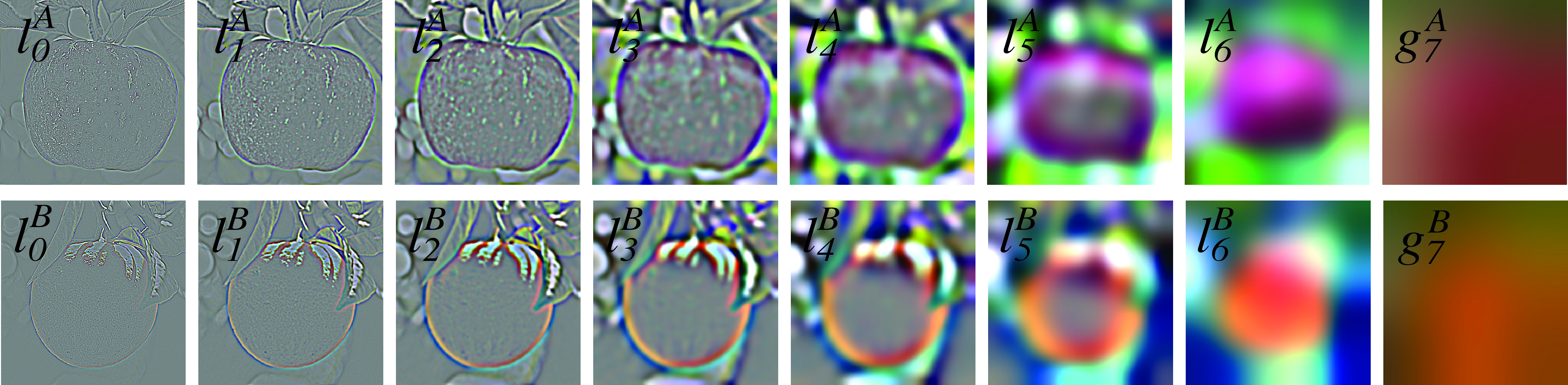
Using the Laplacian pyramid, we can transition from one image to the next over many different spatial scales to make a gradual transition between the two images. The algorithm proceeds as follows. We first build the Laplacian pyramid for the two input images; in this example we use seven levels and we also keep the last low-pass residual as shown in Figure 23.8.
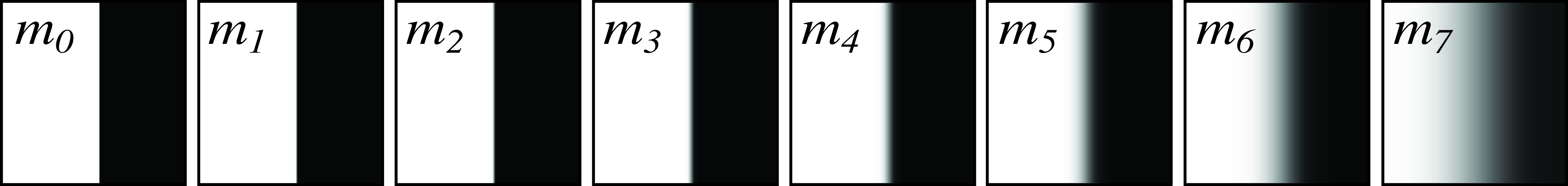
The second step is to build the Gaussian pyramid of the mask as shown in Figure 23.9 (note that we use eight levels, one level more than for the Laplacian pyramid).
In the third step, we combine the three pyramids to compute the Laplacian pyramid of the blended image. The Laplacian pyramid of the blended image is obtained as \[\mathbf{l}_k = \mathbf{l}_k^A * \mathbf{m}_k + \mathbf{l}_i^B * (1-\mathbf{m}_k)\] The same is done for the low-pass residual.
Finally, the fourth step consists in collapsing (i.e., decoding) the resulting pyramid to produce the blended image shown in Figure 23.10.
The result in Figure 23.10 has a smooth transition between the two sides and produces a pleasing blending. The mask does no need to be rectangular. It is possible to blend arbitrary images with complex masks, but the quality of the final image will depend on how well aligned the images are and the composition of the objects in the scene. This is method remains one of the most popular methods for image blending due to its simplicity and the quality of the resulting images.
This method will fail when blending requires geometric image transformations.
23.6 Steerable Pyramid
The Laplacian pyramid provides a richer representation than the Gaussian pyramid. But we would like to have an even more expressive image representation. The steerable pyramid [3] adds information about image orientation. Therefore, the steerable representation is a multiscale oriented representation that is translation-invariant. It is non-aliased and self-invertible. Ideally, we’d like to have an image transformation that was shiftable, that is, where we could perform interpolations in position, scale, and orientation using linear combinations of a set of basis coefficients.
We analyze in orientation using a steerable filter bank, shown in Figure 23.11. We form a decomposition in scale by introducing a low-pass filter (designed to work with the selected bandpass filters), and recursively breaking the low-pass filtered component into angular and low-pass frequency components. Pyramid subsampling steps are preceded by sufficient low-pass filtering to remove aliasing.
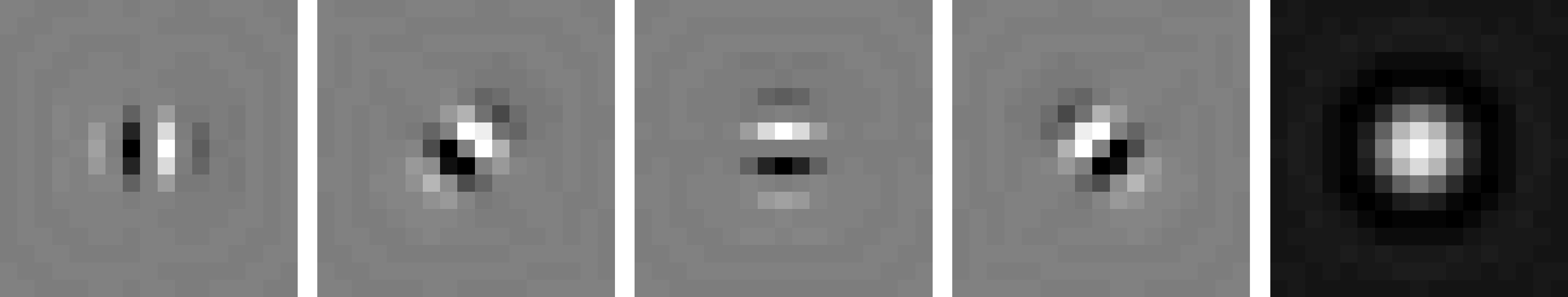
One block of the steerable pyramid computation. 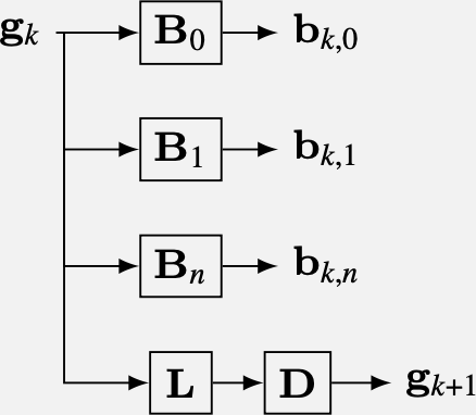
To ensure that the image can be reconstructed from the steerable filter transform coefficients, the filters must be designed so that their sums of squared magnitudes tile in the frequency domain. We reconstruct by applying each filter a second time to the steerable filter representation, and we want the final system frequency response to be flat, for perfect reconstruction.
The following block diagram (Figure 23.12) shows the steps to build a two-level steerable pyramid and the reconstruction of the input. The architecture has two parts: (1) the analysis network (or encoder) that transforms the input image \(x\) into a representation composed of \(r=\left[ b_{0,0},...,b_{0,n}, b_{1,0},...b_{1,n},...,b_{k-1,0},...b_{k-1,n} \right]\) and the low pass residual \(g_{k-1}\); and (2) the synthesis network (or decoder) that reconstructs the input from the representation \(r\).
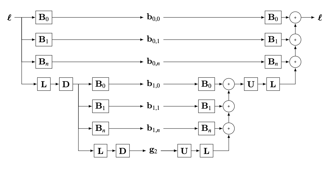
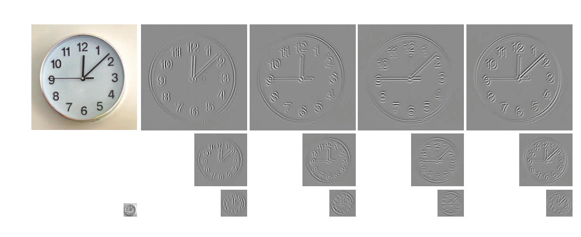
Figure 23.13 shows an example of an image and its steerable pyramid decomposition using four orientations and three scales. The steerable pyramid is a self-inverting overcomplete representation (more coefficients than pixels).
23.7 A Pictorial Summary
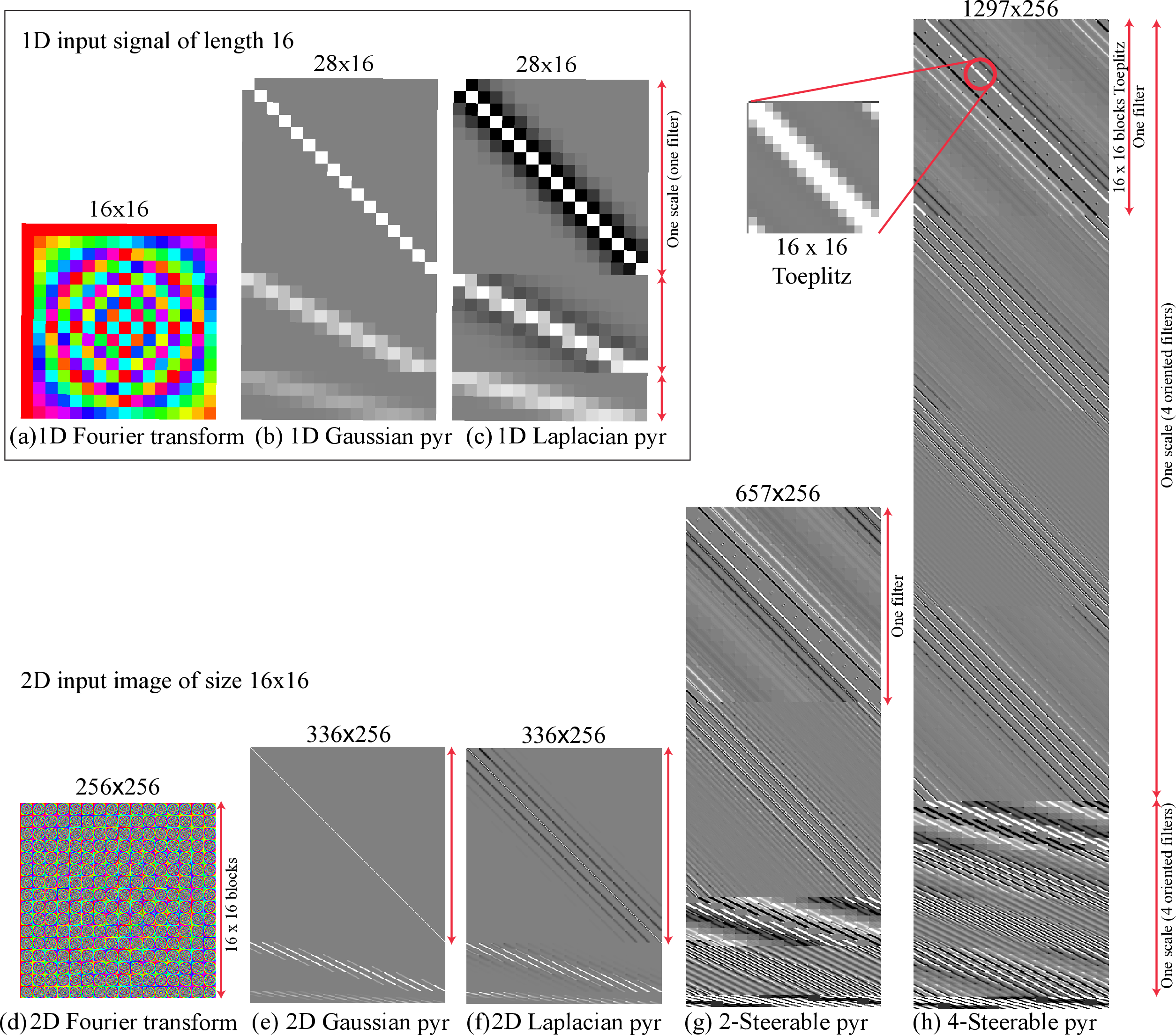
Figure 23.14 shows a pictorial summary of the different pyramid representations we’ve discussed in this chapter. The figure shows the projection matrices \(\mathbf{P}\) for each transformation, both in the 1D case and 2D case. Each projection matrix formed by stacking the projection matrices of each pyramid level.
Figure 23.14 (a-c) start with a 1D input signal of length 16. For instance, for a three-level Gaussian pyramid, Figure 23.14 (b) shows the following projection matrix: \[\mathbf{P} = \begin{bmatrix} \mathbf{I} \\ \mathbf{G}_0 \\ \mathbf{G}_1 \\ \end{bmatrix}\] The first block is the identity matrix as the first level is the input image itself.
For a two-level Laplacian pyramid with a Gaussian residual, the projection matrix \(\mathbf{P}\) is (Figure 23.14[b]): \[\mathbf{P} = \begin{bmatrix} \mathbf{L}_0 \\ \mathbf{L}_1 \\ \mathbf{G}_1 \\ \end{bmatrix}\]
The Fourier transform gives a complex-valued output (represented in color) and is global, that is, each output coefficient depends, in general, on every input pixel. The Gaussian pyramid is seen to be banded, showing that it is a localized transform where the output values only depend on pixels in a neighborhood. It is an overcomplete representation, shown by the transform matrix being taller than it is wide. The Laplacian pyramid is a band-passed image representation, except for the low-pass residual layer, shown in the bottom rows. For this matrix, zero is plotted as gray.
Figures Figure 23.14 (d-h) show the projection matrices when the input is a 2D image of size 16×16 pixels. First, the image is represented as a column vector of length 256=16×16 values. Figure 23.14 (d) shows the projection matrix of the 2D Fourier transform, a square matrix of size 256×256, composed of small blocks of size 16×16 that look like 1D Fourier transforms. Figures Figure 23.14 (e and f) show the Gaussian and Laplacian pyramids, respectively.
Figures Figure 23.14 (g-h) show the steerable pyramid representation, depending on the number of orientations (Figure 23.14 g is a pyramid with two orientations and Figure 23.14 h has four orientations per scale). The steerable pyramid representation can be very overcomplete (the matrix is much taller than wide).
The steerable pyramid is an overcomplete, multiorientation representation. We only show the stererable pyramid for 2D images as in 1D, image orientation isn’t defined. The multiple orientations, and non-aliased subbands cause the representation to be very overcomplete, much taller than it is wide. The last block of the steerable pyramid projection matrices computes the low-pass residual.
23.8 Concluding Remarks
To recap briefly, the Fourier transform reveals spatial frequency content of the image wonderfully, but suffers from having no spatial localization. A Gaussian pyramid provides a multiscale representation of the image, useful for applying a fixed-scale algorithm to an image over a range of spatial scales. But it doesn’t break the image into finer components than simply a range of low-pass filtered versions. The representation is overcomplete that is, there are more pixels in the Gaussian pyramid representation of an image than there are in the image itself.
The Laplacian pyramid reveals what is captured at one spatial scale of a Gaussian pyramid, and not seen at the lower-resolution level above it. Like the Gaussian pyramid, it is overcomplete. It is useful for various image manipulation tasks, allowing you to treat different spatial frequency bands separately.
The steerable pyramid adds orientation information into the representation, and the representation can be very overcomplete (the matrix is much taller than wide). The steerable pyramid has negligible aliasing artifacts and so can be useful for various image analysis applications.
In image processing applications (i.e., image compression, denoising, etc.) people have used other transforms. For instance, the Haar/wavelet/QMF pyramid [1] brings in some limited orientation analysis and different than the other pyramid representations, is complete rather than overcomplete. This helps it for image compression applications, but hurts it for others because each subband depends on information in other subbands to let it reconstruct the original image without artifacts. So if you alter one band without altering the corresponding other ones, you can easily introduce artifacts (although artifacts will also appear in overcompleted representations).
Another important framework for multiscale image analysis, not presented in this book, is scale space. For an in-depth presentation of this topic, we direct the reader to [4].