18 Image Derivatives
18.1 Introduction
Computing image derivatives is an essential operator for extracting useful information from images. As we show in the previous chapter, image derivatives allowed us to compute boundaries between objects and to have access to some of the three-dimensional (3D) information lost when projecting the 3D world into the camera plane. Derivatives are useful because they give us information about where changes are happening in the image, and we expect those changes to be correlated with transitions between objects.
The operator that computes the image derivatives along the spatial dimensions (\(x\) and \(y\)) is a linear system:
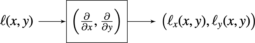
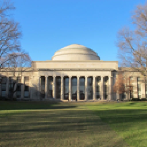
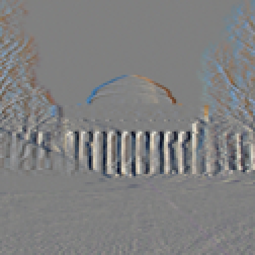
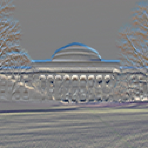
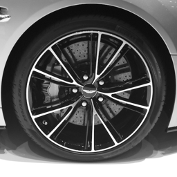
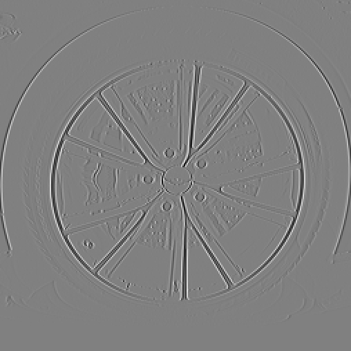
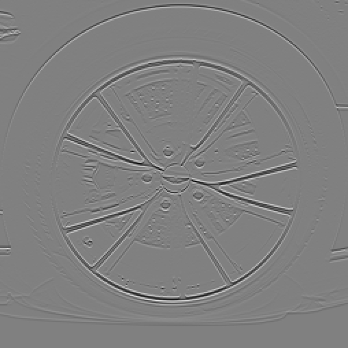
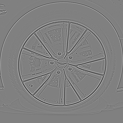
The derivative operator is linear and translation invariant. Therefore, it can be written as a convolution. The following images show an input image and the resulting derivatives along the horizontal and vertical dimensions using one of the discrete approximations that we will discuss in this chapter.
18.2 Discretizing Image Derivatives
If we had access to the continuous image, then image derivatives could be computed as: \(\partial \ell (x,y) / \partial x\), which is defined as:
\[ \frac{\partial \ell(x,y)} {\partial x} = \lim_{\epsilon \to 0} \frac{ \ell(x+\epsilon,y) -\ell(x,y)} {\epsilon} \]
However, there are several reasons why we might not be able to apply this definition:
- We only have access to a sampled version of the input image, \(\ell \left[n,m\right]\), and we cannot compute the limit when \(\epsilon\) goes to zero.
- The image could contain many non-derivable points, and the gradient would not be defined. We will see how to address this issue later when we study Gaussian derivatives.
- In the presence of noise, the image derivative might not be meaningful as it might just be dominated by the noise and not by the image content.
For now, let’s focus on the problem of approximating the continuous derivative with discrete operators. As the derivative is a linear operator, it can be approximated by a discrete linear filter. There are several ways in which image derivatives can be approximated.
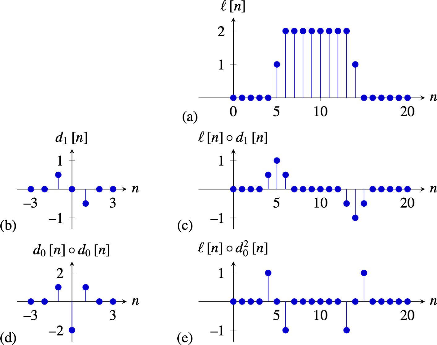
Let’s start with a simple approximation to the derivative operator that we have already played with \(d_0 = \left[1, -1 \right]\). In one dimension (1D), convolving a signal \(\ell \left[n \right]\) with this filter results in: \[ \ell \circ d_0 = \ell \left[n \right] - \ell \left[n-1 \right] \] This approximates the derivative by the difference between consecutive values, which is obtained when \(\epsilon=1\). Figure 18.3 (c) shows the result of filtering a 1D signal (Figure 18.3) convolved with \(d_0 \left[n\right]\) (Figure 18.3). The output is zero wherever the input signal is constant, and it is large in the places where there are variations in the input values. However, note that the output is not perfectly aligned with the input. In fact, there is half a sample displacement to the right. This is due to the fact that \(d_0 \left[n\right]\) is not centered around the origin.
This can be addressed with a different approximation to the spatial derivative \(d_1 = \left[1, 0, -1 \right]/2\). In one dimension, convolving a signal \(\ell \left[n \right]\) with \(d_1 \left[n\right]\) results in: \[ \ell \circ d_1 = \frac{\ell \left[n+1 \right] - \ell \left[n-1 \right]}{2} \] Figure 18.3 (e) shows the result of filtering the 1D signal (Figure 18.3) convolved with \(d_1 \left[n\right]\) (Figure 18.3). Now the output shows the highest magnitude output in the midpoint where there is variation in the input signal.

It is also interesting to see the behavior of the derivative and its discrete approximations in the Fourier domain. In the continuous domain, the relationship between the Fourier transform on a function and the Fourier transform of its derivative is: \[ \frac{\partial \ell (x)}{\partial x} \xrightarrow{\mathscr{F}} j w \mathscr{L} (w) \] In the continuous Fourier domain, derivation is equivalent to multiplying by \(jw\). In the discrete domain, the DFT of a signal derivative will depend on the approximation used. Let’s study now the DFT of the two approximations that we have discussed here, \(d_0\) and \(d_1\).
The DFT of \(d_0 \left[n\right]\) is: \[ \begin{split} D_0 \left[u \right] & = 1 - \exp \left( -2 \pi j \frac{u}{N} \right) \\ & = \exp \left( - \pi j \frac{u}{N} \right) \left( \exp \left( \pi j \frac{u}{N} \right) - \exp \left( -\pi j \frac{u}{N} \right) \right) \\ & = \exp \left( - \pi j \frac{u}{N} \right) 2 j \sin (\pi u /N) \end{split} \] The first term is a pure phase shift, and it is responsible for the half a sample delay in the output. The second term is the amplitude gain, and it can be approximated by a linear dependency on \(u\) for small \(u\) values.
The DFT of \(d_1 \left[n\right]\) is: \[ \begin{split} D_1 \left[u \right] & = 1/2\exp \left( 2 \pi j \frac{u}{N} \right) - 1/2 \exp \left( -2 \pi j \frac{u}{N} \right) \\ & = j \sin (2 \pi u /N) \end{split} \]
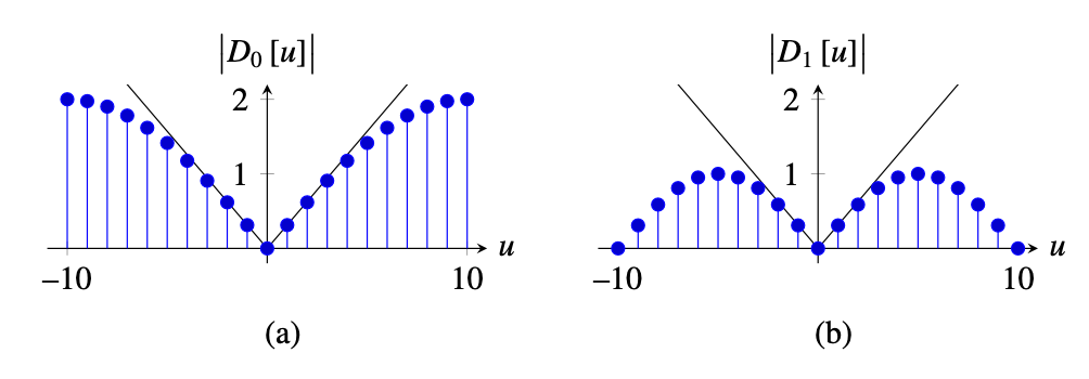
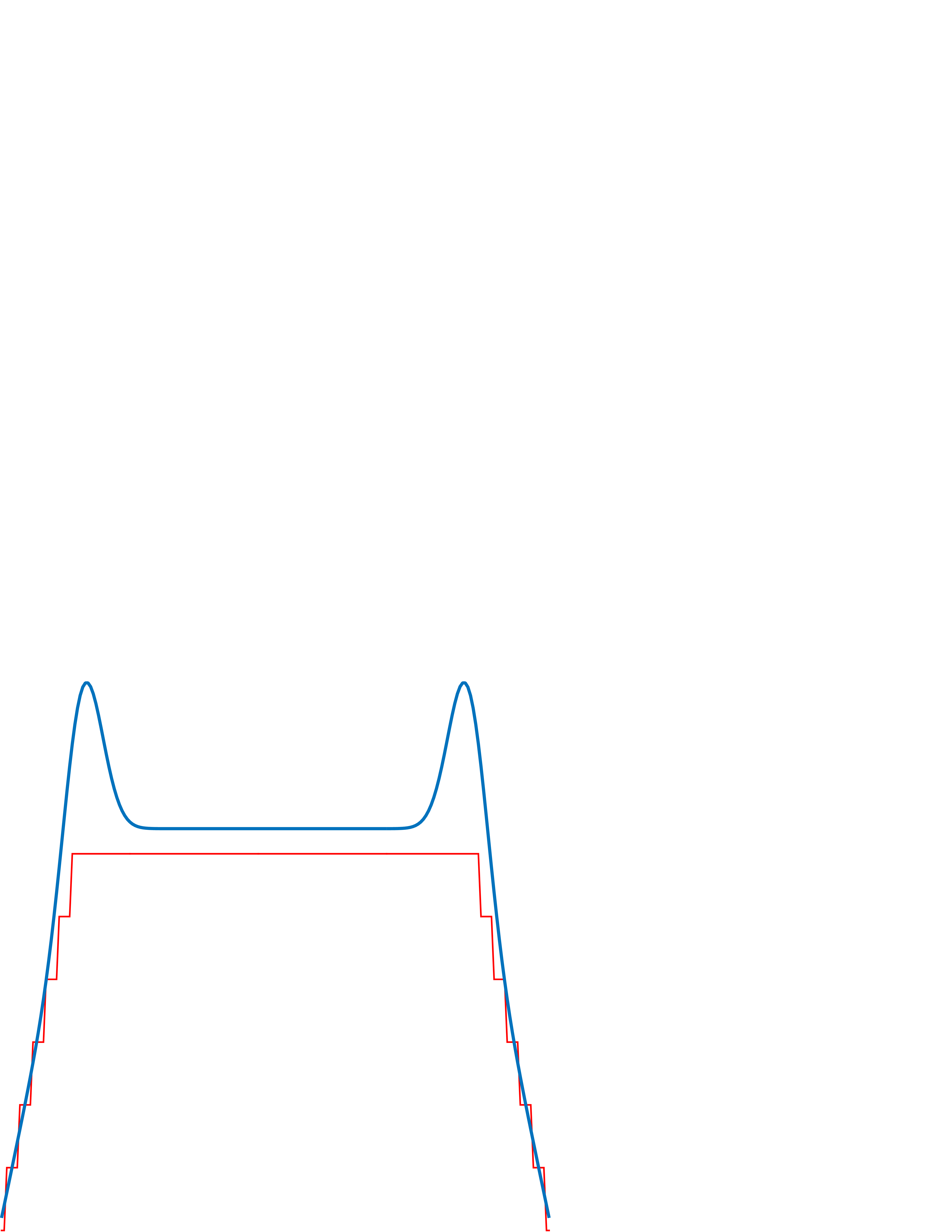
Figure 18.4 shows the magnitude of \(D_0\left[u \right]\) and \(D_1\left[u \right]\) and compares it with \(\left| 2 \pi u/N \right|\), which will be the ideal approximation to the derivative. The amplitude of \(D_0\left[u \right]\) provides a better approximation to the ideal derivative, but the phase of \(D_0\left[u \right]\) introduces a small shift in the output. Conversely, \(D_1\left[u \right]\) has no shift, but it approximates the derivative over a smaller range of frequencies. The output to \(D_1\left[u \right]\) is smoother than the output to \(D_0\left[u \right]\), and, in particular, \(D_1\left[u \right]\) gives a zero output when the input is the signal \(\left[ 1, -1, 1, -1, ... \right]\). In fact, we can see that \(\left[1,0,-1\right] = \left[1,-1\right] \circ \left[1,1\right]\), and, therefore \(D_1\left[u \right] = D_0\left[u \right] B_1\left[u \right]\), where \(B_1\left[u \right]\) is the DFT of the binomial filter \(b_1 \left[n \right]\).
When working with two-dimensional (2D) images, there are several ways in which partial image derivatives can be approximated. For instance, we can compute derivatives along
the \(n\) and \(m\) components:
\[ \begin{bmatrix} 1 \\ -1 \end{bmatrix} ~~~~~~~ \begin{bmatrix} 1 & -1 \end{bmatrix} \] The problem with this discretization of the image derivatives is that the outputs are spatially misaligned because a filter of length 2 shifts the output image by half a pixel as we discussed earlier. The spatial misalignment can be removed by using a slightly different version of the same operator: we can use a rotated reference frame as it is done in the Roberts cross operator, introduced in 1963 [1] in a time when reading an image of \(256 \times 256\) pixels into memory took several minutes:
\[ \begin{bmatrix} 1 & ~0\\ 0 & -1 \end{bmatrix} ~~~~~~~ \begin{bmatrix} ~0 & 1 \\ -1 & 0 \end{bmatrix} \] Now, both outputs are spatially aligned because they are shifted in the same way. Another discretization is the Sobel operator, based on the \([-1,0,1]\) kernel, and will be discussed in Section 18.7.
While newer algorithms for edge extraction have been developed since the creation of these operators, they still hold value in cases where efficiency is important. These simple operators continue to be used as fundamental components in modern computer vision descriptors, including the Scale-invariant feature transform (SIFT) [2] and the histogram of oriented gradients (HOG) [3].
18.3 Gradient-Based Image Representation
Derivatives have become an important tool to represent images, and they can be used to extract a great deal of information from the image as it was shown in the previous chapter. One thing about derivatives is that it might seem as though we are losing information from the input image. An important question is if we have the derivative of a signal, can we recover the original image? What information is being lost? Intuitively, we should be able to recover the input image by integrating its derivative, but it is an interesting exercise to look in detail at how this integration can be performed. We will start with a 1D signal, and then we will discuss the 2D case.
A simple way of seeing that we can recover the input from its derivatives is to write the derivative in matrix form. This is the matrix that corresponds to the convolution with the kernel \(\left[1, -1 \right]\) that we will call \(\mathbf{D_0}\). The next two matrices show the matrix \(\mathbf{D_0}\) and its inverse \(\mathbf{D_0}^{-1}\) for a 1D image of length five pixels using zero boundary conditions:
\[ \mathbf{D_0} = \begin{bmatrix} 1 ~& 0 ~& 0 ~& 0~& 0 \\ -1 ~& 1 ~& 0 ~& 0~& 0 \\ 0 ~& -1 ~& 1 ~& 0 ~& 0\\ 0~& 0 ~& -1 ~& 1 ~& 0\\ 0~& 0 ~& 0 ~& -1 ~& 1 \end{bmatrix} ~~~~~~~~~ \mathbf{D_0}^{-1} = \begin{bmatrix} 1 ~&~ 0 ~&~ 0 ~&~ 0~&~ 0 \\ 1 ~&~ 1 ~&~ 0 ~&~ 0~&~ 0 \\ 1 ~&~ 1 ~&~ 1 ~&~ 0 ~&~ 0\\ 1~&~ 1 ~&~ 1 ~&~ 1 ~&~ 0\\ 1~&~ 1 ~&~ 1 ~&~ 1 ~&~ 1 \end{bmatrix} \] We can see that the inverse \(\mathbf{D_0}^{-1}\) is reconstructing each pixel as a sum of all the derivative values from the left-most pixel to the right. And the inverse perfectly reconstructs the input. But, this is cheating because the first sample of the derivative gets to see the actual value of the input signal, and then we can integrate back the entire signal. That matrix is assuming zero boundary conditions for the signal, and the boundary gives us the needed constraint to be able to integrate back the input signal.
But what happens if you only get to see valid differences and you remove any pixel that was affected by the boundary? In this case, the derivative operator in matrix form is:
\[ \mathbf{D_0} = \begin{bmatrix} -1 ~& 1 ~& 0 ~& 0~& 0 \\ 0 ~& -1 ~& 1 ~& 0 ~& 0\\ 0~& 0 ~& -1 ~& 1 ~& 0\\ 0~& 0 ~& 0 ~& -1 ~& 1 \end{bmatrix} \]
Let’s consider the next 1D input signal:
\[ \boldsymbol\ell = \left[1, 1, 2, 2, 0\right] \]
Then, the output of the derivative operator is:
\[ \mathbf{r}=\mathbf{D_0} \boldsymbol\ell=\left[0, -1, 0, 2\right] \] Note that this vector has one sample less than the input. To recover the input \(\boldsymbol\ell\) we cannot invert \(\mathbf{D_0}\) as it is not a square matrix, but we can compute the pseudoinverse, which turns out to be:
\[ \mathbf{D_0}^{+} = \frac{1}{5} \begin{bmatrix} -4 ~& -3 ~& -2~& -1 \\ 1 ~& -3 ~& -2 ~&-1 \\ 1~& 2 ~& -2 ~& -1\\ 1~& 2 ~& 3 ~& -1\\ 1~& 2 ~& 3 ~& 4 \end{bmatrix} \] The pseudoinverse has an interesting structure, and it is easy to see how it can be written in the general form for signals of length \(N\). Also, note that \(\mathbf{D_0}^{+}\) cannot be written as a convolution. Another important thing is that the inversion process is trying to recover more samples than there are observations. The trade-off is that the signal that it will recover will have zero mean (so it loses one degree of freedom that cannot be estimated). In this example, the reconstructed input is:
\[ \hat{\boldsymbol\ell} = \mathbf{D_0}^{+} \mathbf{r} = \left[-0.2, -0.2, 0.8, 0.8, -1.2 \right] \] Note that \(\hat{\boldsymbol\ell}\) is a zero mean vector. In fact, the recovered input is a shifted version of the original input, \(\hat{\boldsymbol\ell} = \boldsymbol\ell - 1.2\), where 1.2 is the mean value of samples on \(\boldsymbol\ell\). Then, you still can recover the input signal up to the DC component (mean signal value).
18.4 Image Editing in the Gradient Domain
One of the interests of transforming an image into a different representation than pixels is that it allows us to manipulate aspects of the image that would be hard to control using the pixels directly. Figure 18.5 shows an example of image editing using derivatives.
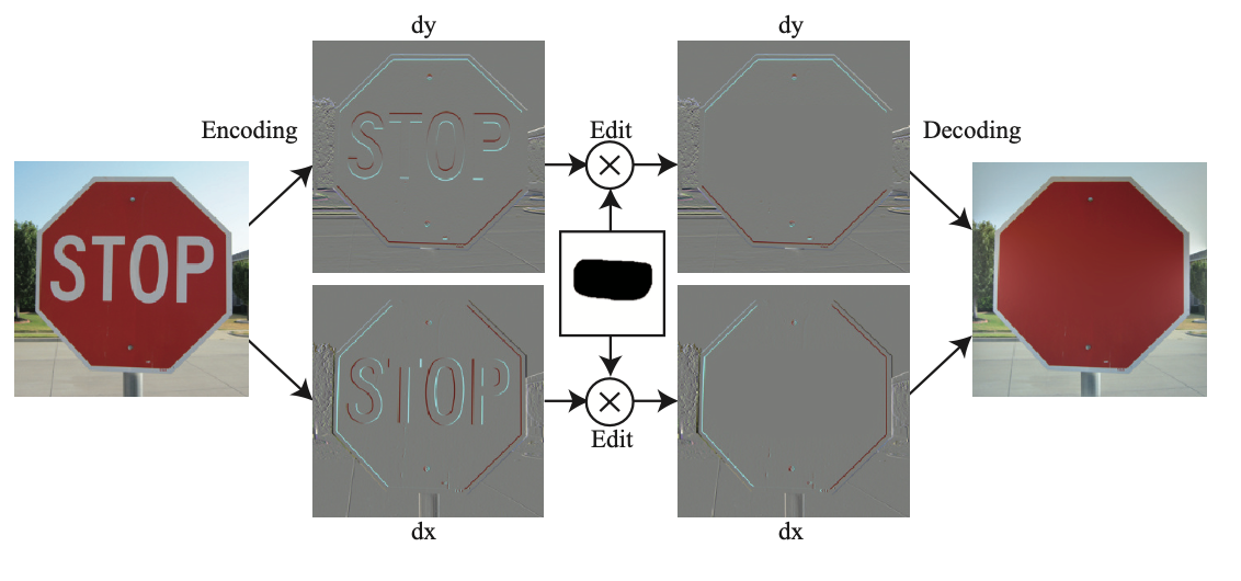
First, the image is encoded using derivatives along the \(x\) and \(y\) dimensions: \[ \mathbf{r} = \left[ \begin{array}{c} \mathbf{D_x} \\ \mathbf{D_y} \end{array} \right] \boldsymbol\ell \] The resulting representation, \(\mathbf{r}\), contains the concatenation of the output of both derivative operators. \(\mathbf{r}\) will have high values in the image regions that contain changes in pixel intensities and colors and will be near zero in regions with small variations. This representation can be decoded back into the input image by using the pseudoinverse as we did in the 1D case. The pseudoinverse can be efficiently computed in the Fourier domain [4].
We can now manipulate this representation. In the example shown in Figure 18.5, if we set to zero the image derivatives that correspond to the word “stop,” when we decode the representation, we obtain a new image where the word “stop” has been removed. The red color fills the region with the word present in the input image.
Image inpainting consists in filling a missing region in an image.
We did not have to specify what color that region had to be; that information comes from the integration process. Therefore, deleting an object using image derivatives can be achieved by setting to zero the gradients regardless of the content that will fill that region. Similarly, we could remove any object in an image or create new textures by modifying its gradient representation.
18.5 Gaussian Derivatives
In the previous sections, we studied how to discretize derivatives and how to use them to represent images. However, computing derivatives in practice presents several difficulties. First, derivatives are sensitive to noise. In the presence of noise, as images tend to vary slowly, the difference between two continuous pixel values will be dominated by noise. This is illustrated in Figure 18.6.
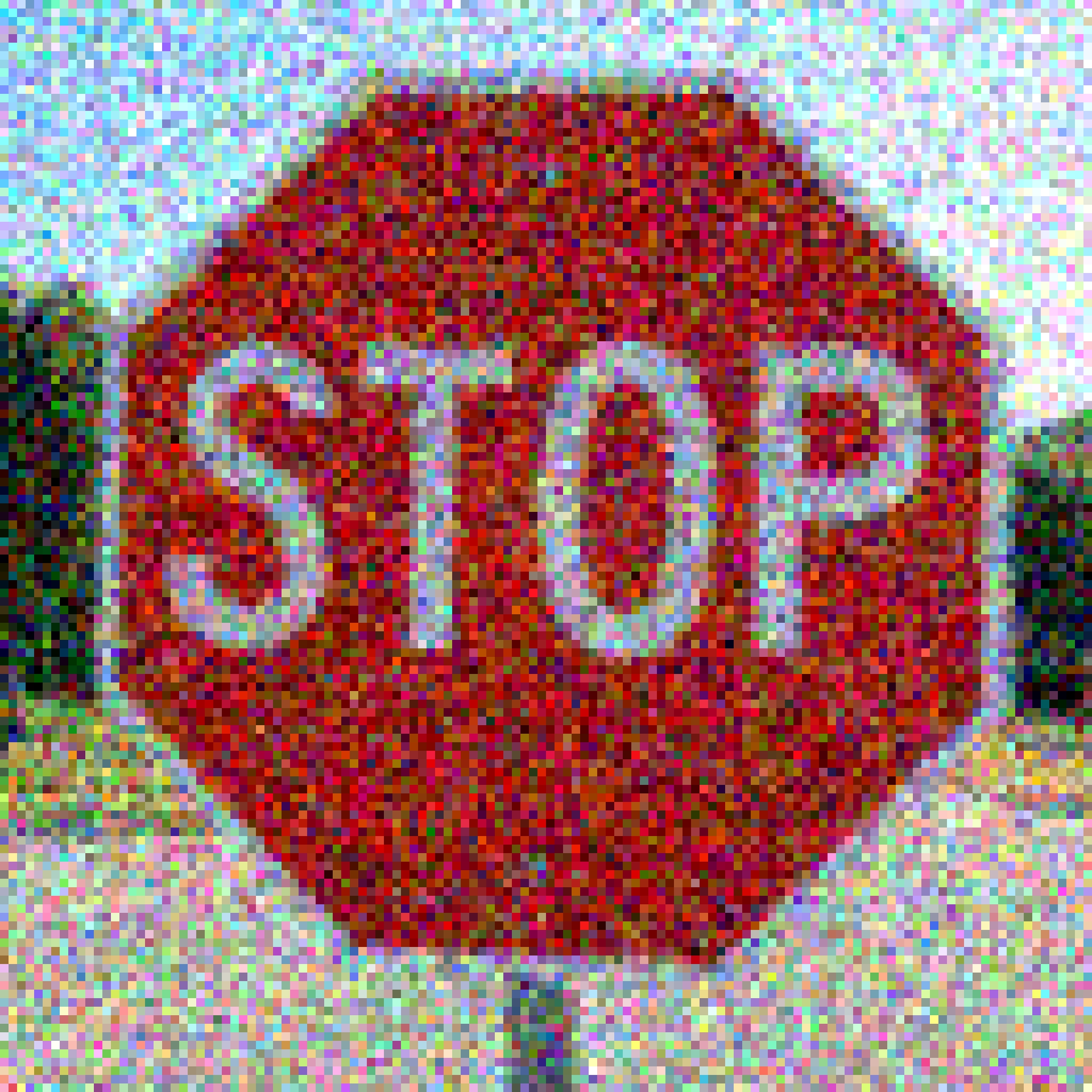

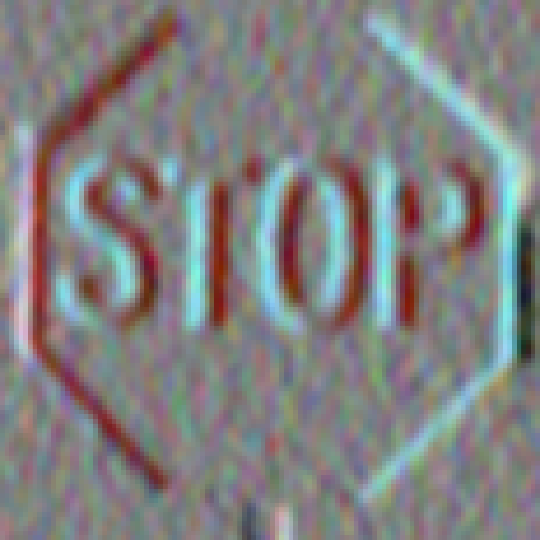
As shown in Figure 18.6, the input is an image corrupted with Gaussian noise. The result of convolving the input noisy image with the kernel \([1, -1]\) results in an output with increased noise. This is because the noise at each pixel is independent of the other, so when computing the difference between two adjacent pixels we get increased noise (the difference between two Gaussian random variables with variance \(\sigma^2\) is a new Gaussian with variance \(2\sigma^2\)). On the other hand, the values of the pixels of the original image are very similar and the difference is a small number (except at the object boundaries). As a consequence, the output is dominated by noise as shown in Figure 18.6 (b).
There are also situations in which the derivative of an image is not defined. For instance, consider an image in the continuous domain with the form \(\ell (x,y) = 0\) if \(x<0\) and 1 otherwise. If we try to compute \(\partial \ell (x,y) / \partial x\), we will get 0 everywhere, but around \(x=0\) the value of the derivative is not defined. We avoided this issue in the previous section because for discrete images the approximation of the derivative is always defined.
Gaussian derivatives address these two issues. They were popularized by Koenderink and Van Doorm [5] as a model of neurons in the visual system.
Let’s start with the following observation. For two functions defined in the continuous domain \(\ell(x,y)\) and \(g(x,y)\), the convolution and the derivative are commutative: \[ \frac {\partial \ell(x,y)}{\partial x} \circ g(x,y) = \ell(x,y) \circ \frac {\partial g(x,y)}{\partial x} \]
This equality is easy to prove in the Fourier domain. If our goal is to compute image derivatives and then blur the output using a differentiable low-pass filter, \(g(x,y)\), then instead of computing the derivative of the image we can compute the derivatives of the filter kernel and convolve it with the image. Even if the derivative of \(\ell(x,y)\) is not defined in some locations (e.g., step boundaries), we can always compute the result of this convolution.
If \(g(x,y)\) is a blurring kernel, it will smooth the derivatives, reducing the output noise at the expense of a loss in spatial resolution (Figure 1). A common smoothing kernel for computing derivatives is the Gaussian kernel. The Gaussian has nice smoothing properties as we discussed in the previous chapter, and it is infinitely differentiable.
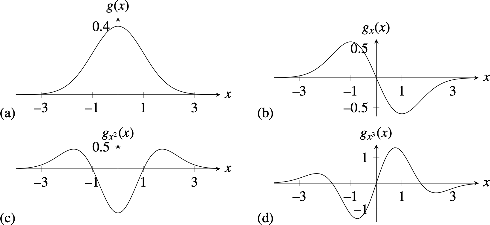
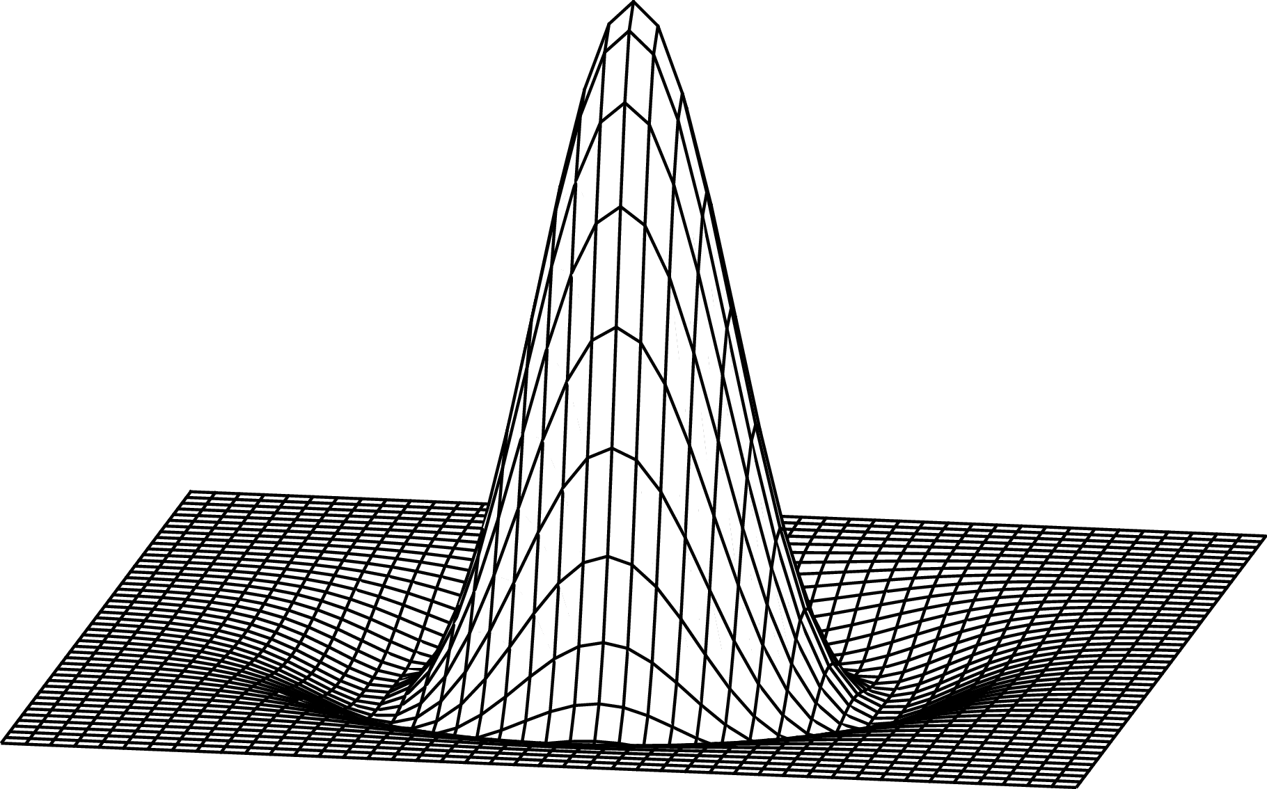
If \(g\) is a Gaussian, then the first-order derivative is \[ \begin{split} g_x(x,y; \sigma) & = \frac {\partial g(x,y; \sigma)}{\partial x} \\ & = \frac{-x}{2 \pi \sigma^4} \exp{-\frac{x^2 + y^2}{2 \sigma^2}} \\ & = \frac{-x}{\sigma^2} g(x,y; \sigma) \end{split} \tag{18.1}\]
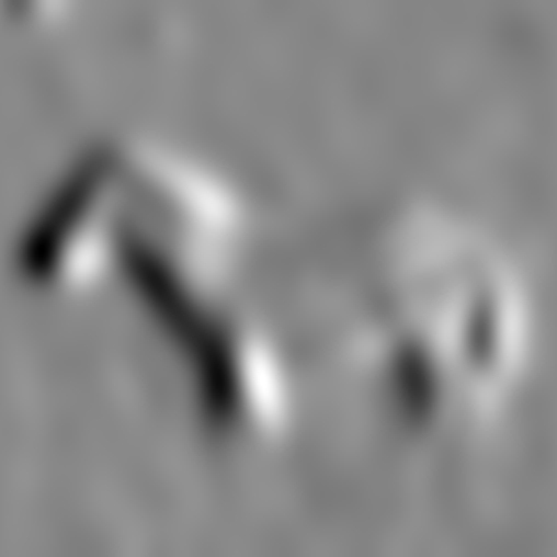
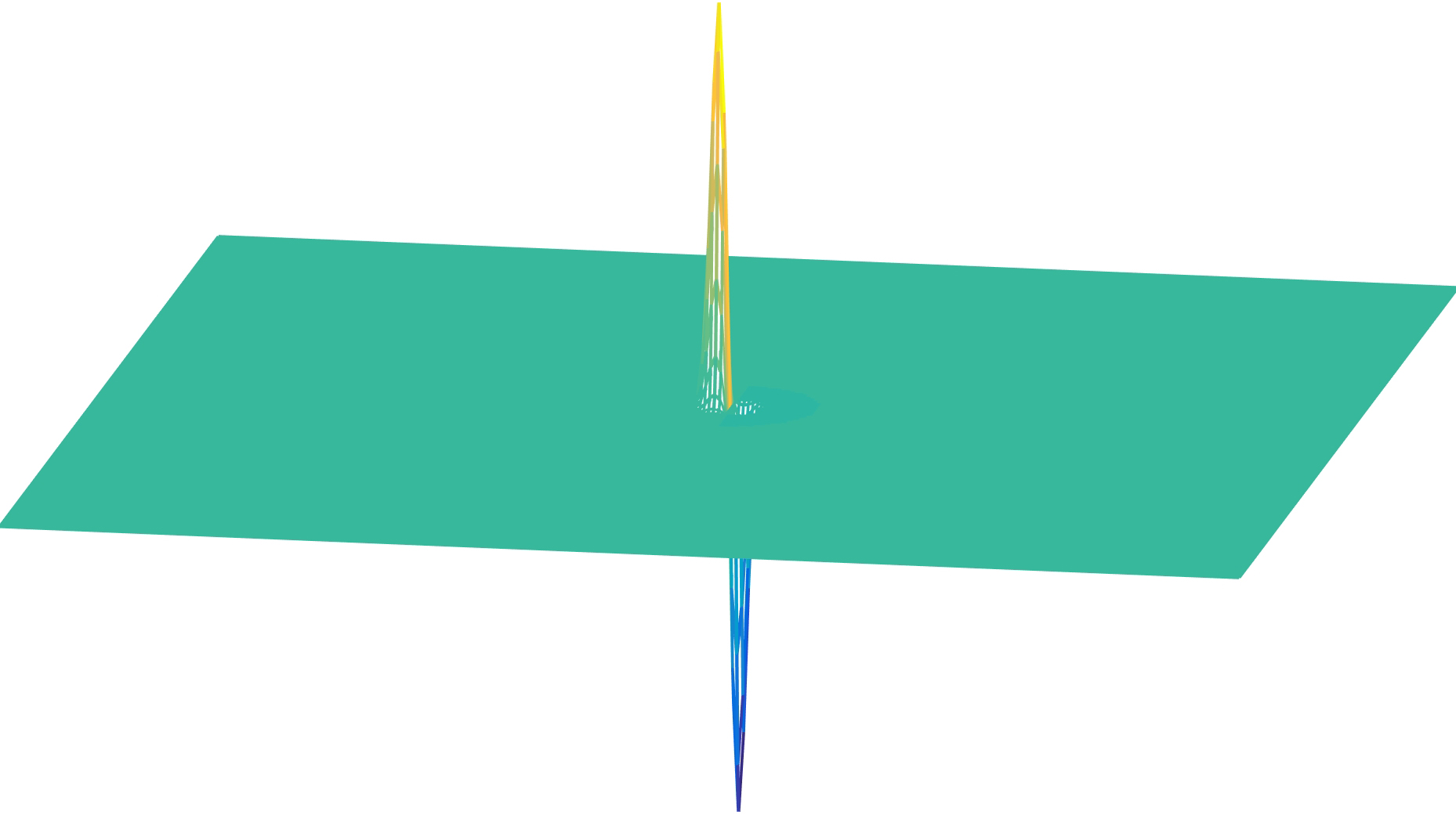
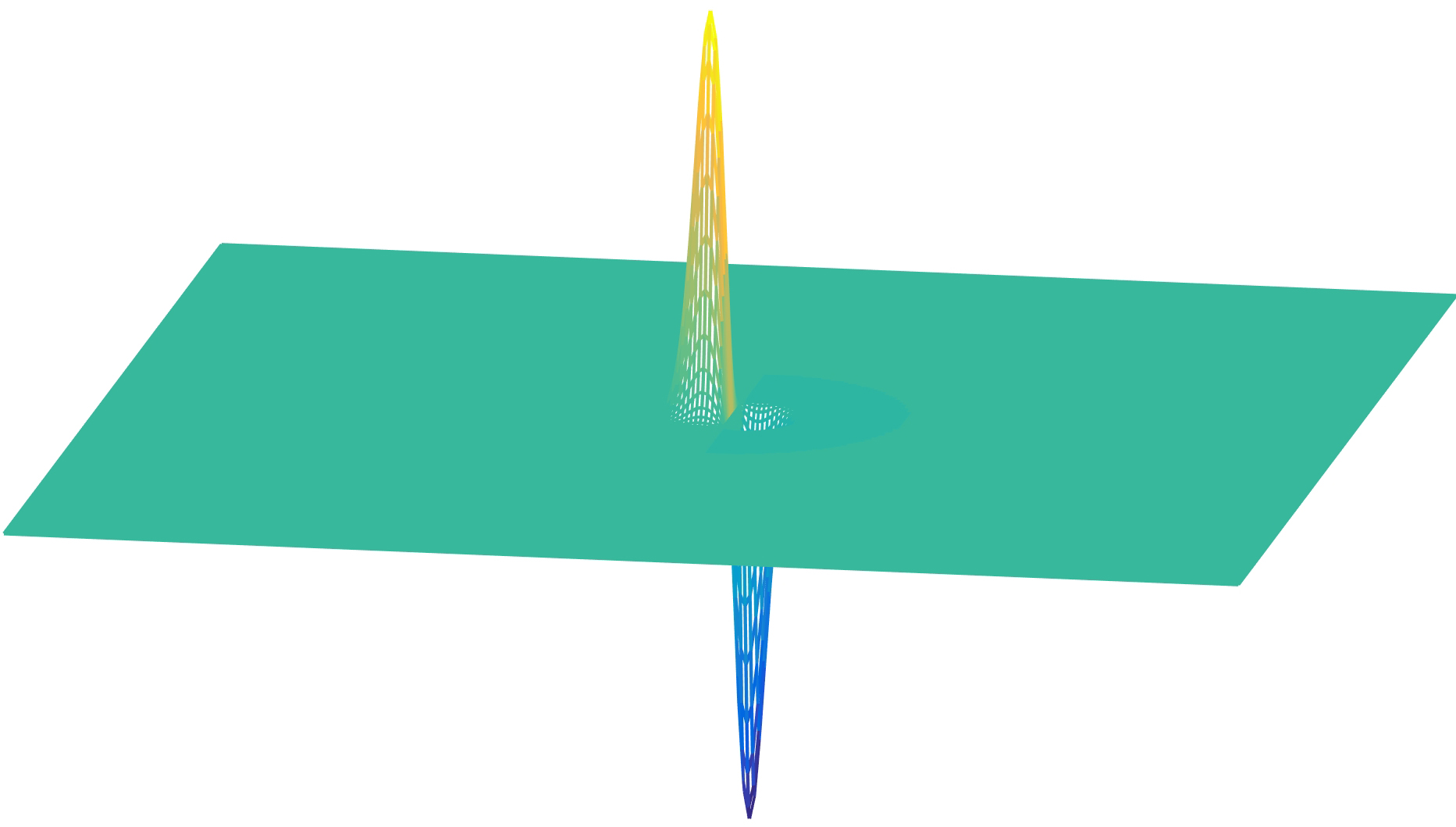
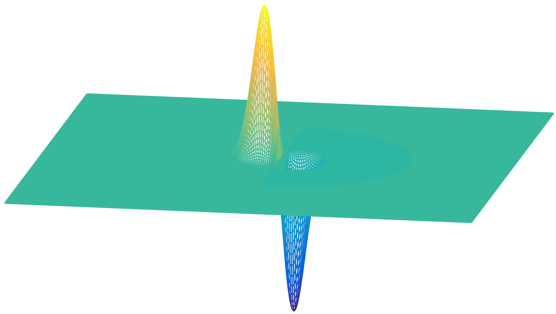
The next plots show the 2D Gaussian with \(\sigma=1\), and its \(x\)-derivative:
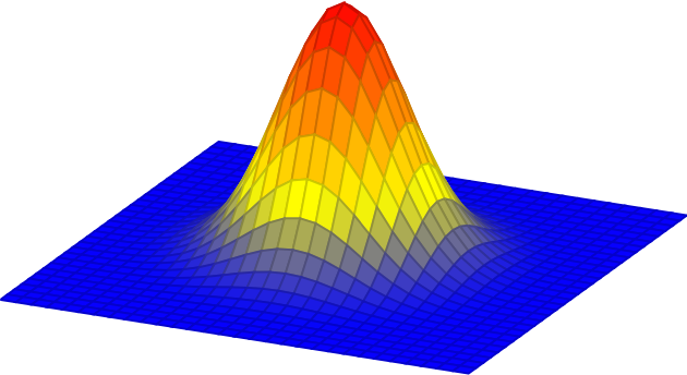
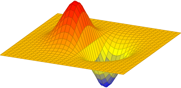
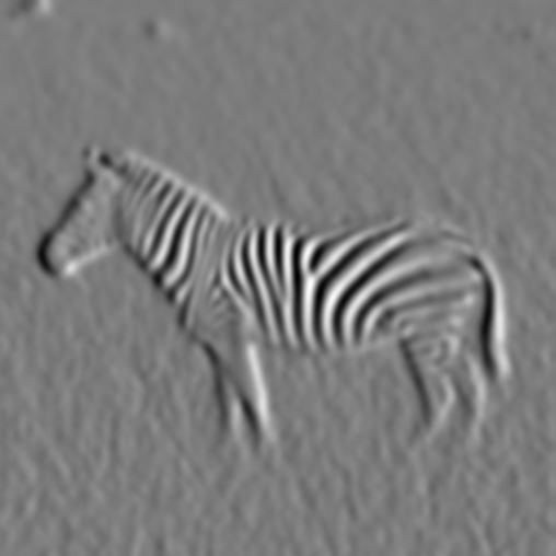
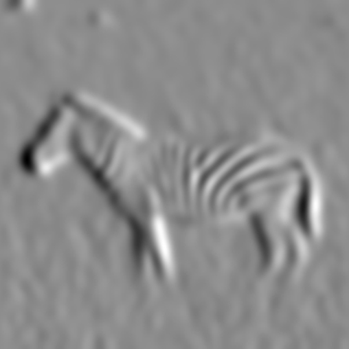
Figure 18.8 shows an image filtered with three Gaussian derivatives with different widths, \(\sigma\). Derivatives at different scales emphasize different aspects of the image. The fine-scale derivatives Figure 18.8 (a) highlight the bands in the zebra, while the coarse-scale derivatives Figure 18.8 (c) emphasize more the object boundaries. This multiscale image analysis will be studied in depth in the following chapter.
18.6 High-Order Gaussian Derivatives
The second-order derivative of a Gaussian is: \[ g_{x^2}(x,y; \sigma) = \frac{x^2-\sigma^2}{\sigma^4} g(x,y; \sigma) \]
The \(n\)-th order derivative of a Gaussian can be written as the product between a polynomial on \(x\), with the same order as the derivative, times a Gaussian. The family of polynomials that result in computing Gaussian derivatives is called Hermite polynomials. The general expression for the \(n\) derivative of a Gaussian is: \[ g_{x^n}(x; \sigma) = \frac{\partial^{n} g(x)}{\partial x^n} = \left( \frac{-1}{\sigma \sqrt{2}} \right)^n H_n\left( \frac{x}{\sigma \sqrt {2}} \right) g(x; \sigma) \] The first Hermite polynomial is \(H_0(x)=1\), the second is \(H_1(x) = 2x\), the third is \(H_2(x)=4x^2-2\), and they can be computed recursively as: \[ H_n(x) = 2x H_{n-1}(x) - 2(n-1)H_{n-2}(x) \]
For \(n=0\) we have the original Gaussian. Figure 18.9 shows the 1D Gaussian derivatives.
In two dimensions, as the Gaussian is separable, the partial derivatives result on the product of two Hermite polynomial, one for each spatial dimension:
\[ \begin{split} g_{x^n,y^m}(x,y; \sigma) & = \frac{\partial^{n+m} g(x,y)}{\partial x^n \partial y^m} \\ & = \left( \frac{-1}{\sigma \sqrt{2}} \right)^{n+m} H_n\left( \frac{x}{\sigma \sqrt {2}} \right) H_m\left( \frac{y}{\sigma \sqrt {2}} \right) g(x,y; \sigma) \end{split} \tag{18.2}\]
Figure 18.10 shows the 2D Gaussian derivatives, and Figure 18.11 shows the corresponding Fourier transforms.
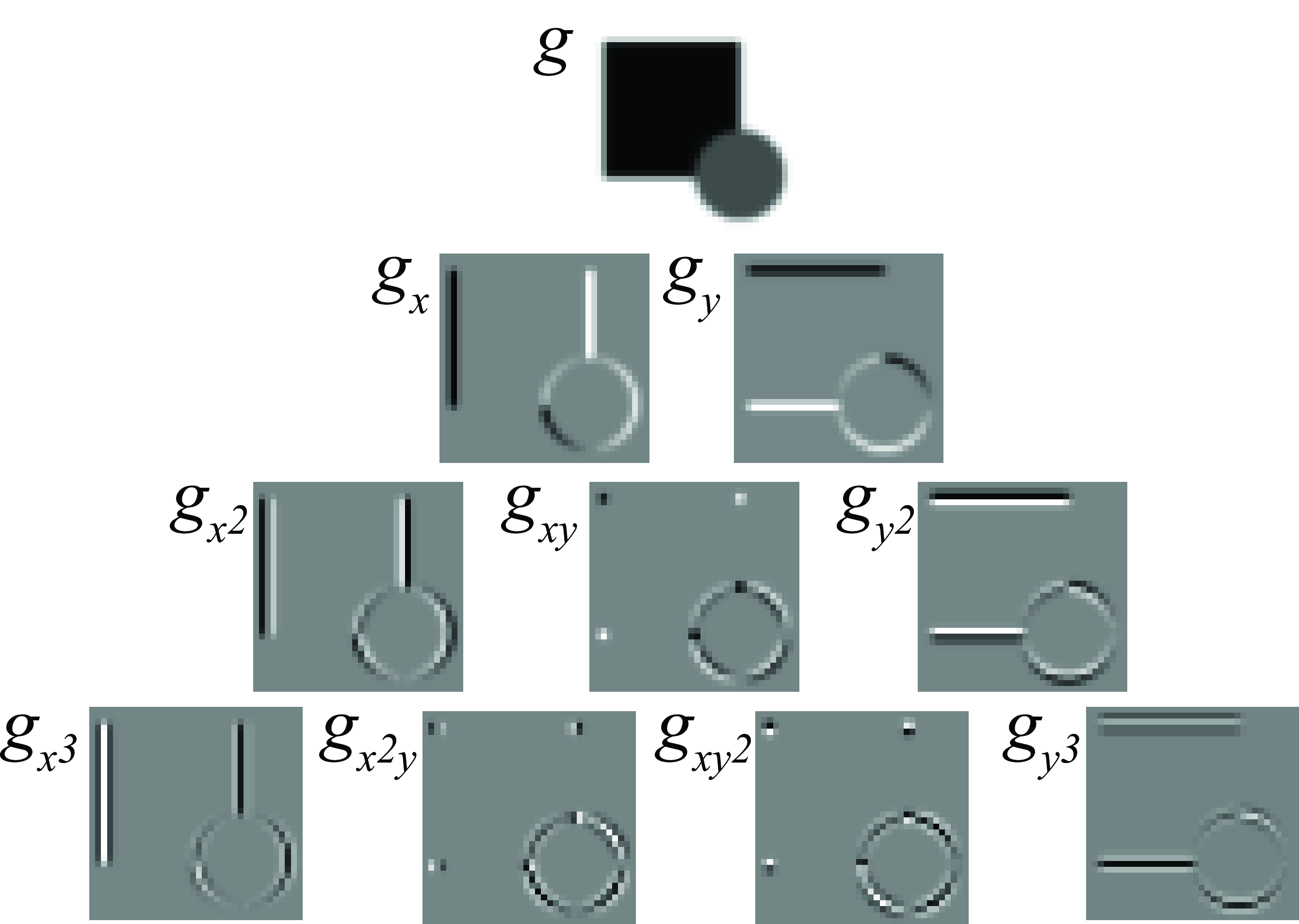
Figure 18.12 shows the output of the derivatives when applied to a simple input image containing a square and a circle. Different derivatives detect a diverse set of image features. However, this representation might not be very useful as it is not rotationally invariant.
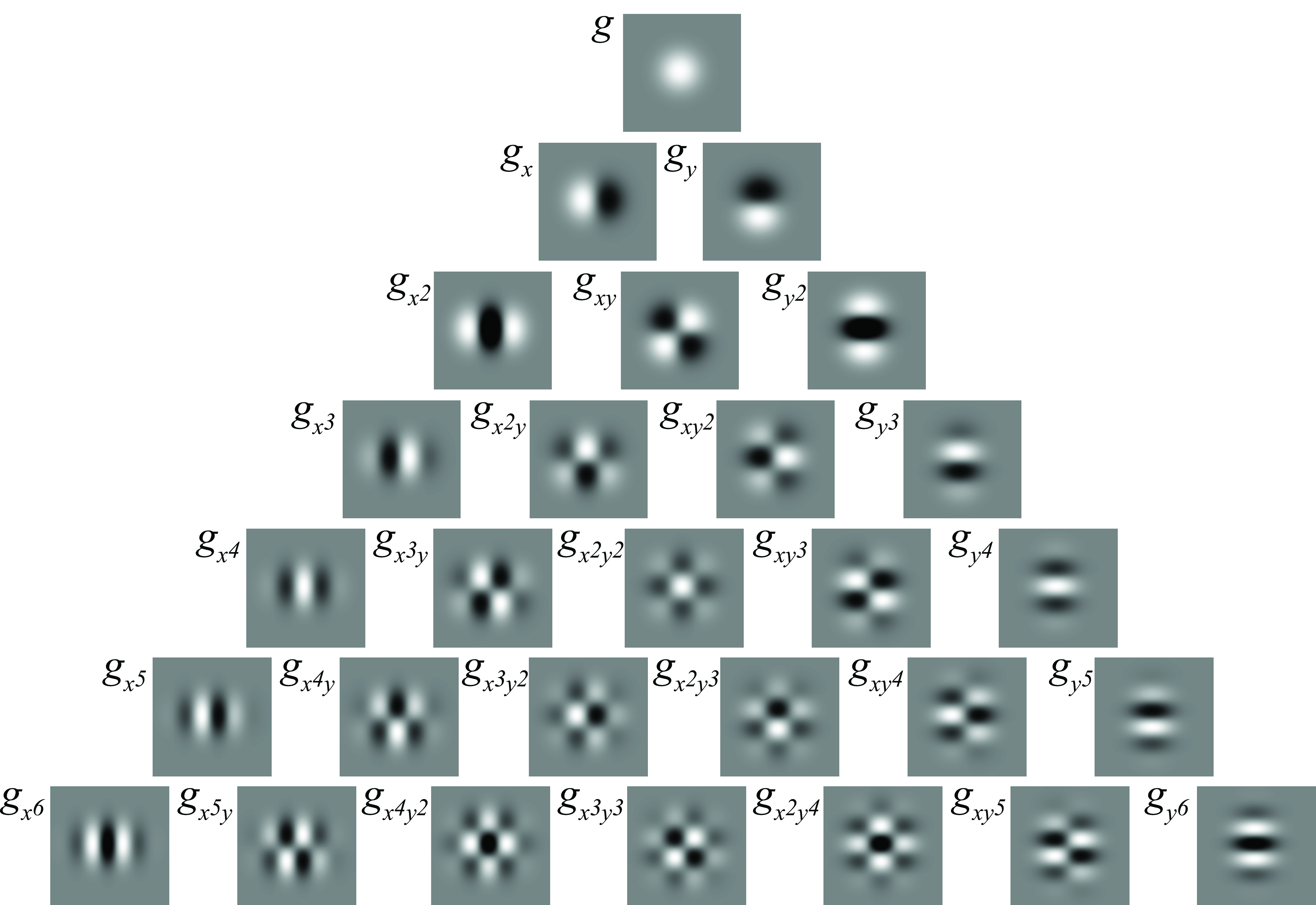
Figure 18.11 shows that they are different from sine and cosine waves; instead, they look more like products of cosine and sine waves.
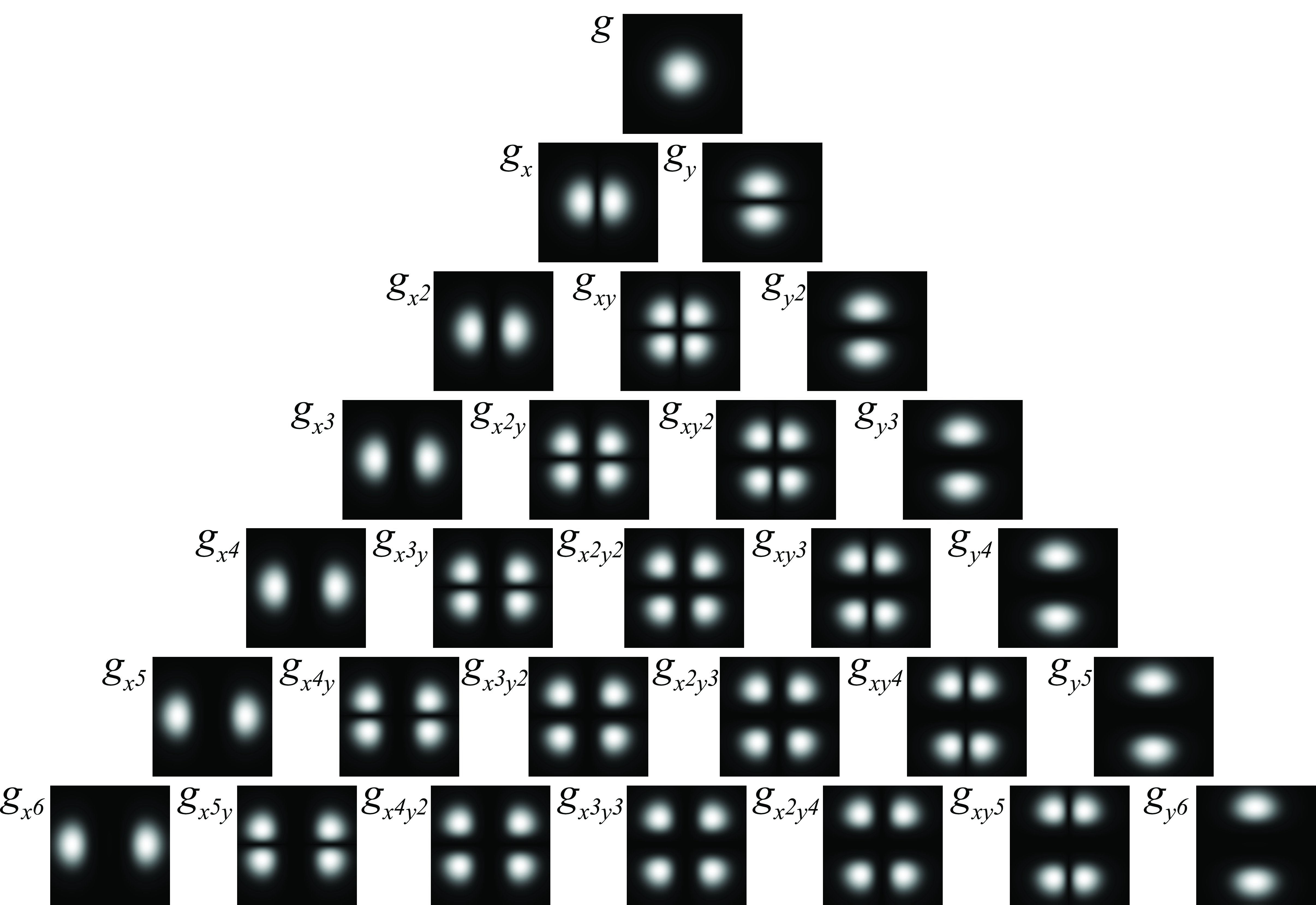
The Gaussian derivatives share many of the properties of the Gaussian. The convolution of two Gaussian derivatives of order \(n\) and \(m\) and variances \(\sigma_1^2\) and \(\sigma_2^2\) result in another Gaussian derivative of order \(n+m\) and variance \(\sigma_1^2 + \sigma_2^2\). Proving this property on the spatial domain can be tedious. However, it is trivial to prove it in the Fourier domain.
18.7 Derivatives using Binomial Filters
When processing images we have to use discrete approximations for the Gaussian derivatives. After discretization, many of the properties of the continuous Gaussian will not hold exactly.
There are many discrete approximations. For instance, we can take samples of the continuous functions. In practice it is common to use the discrete approximation given by the binomial filters. Figure 18.13 shows the result of convolving the binomial coefficients, \(b_n\), with \(\left[1, -1\right]\).
In two dimensions, we can use separable filters and build a partial derivative as:
\[ Sobel_x = \begin{bmatrix} 1 & 0 & -1 \\ \end{bmatrix} \circ \begin{bmatrix} 1 \\ 2 \\ 1 \end{bmatrix} = \begin{bmatrix} 1 & 0 & -1 \\ 2 & 0 & -2 \\ 1 & 0 & -1 \end{bmatrix} \]
\[ Sobel_y = \begin{bmatrix} -1 & -2 & -1 \\ 0 & 0 & 0 \\ 1 & 2 & 1 \end{bmatrix} \tag{18.3}\]
This particular filter is called the Sobel-Feldman operator.
The goal of this operator was to be compact and as isotropic as possible. The Sobel-Feldman operator can be implemented very efficiently as it can be written as the convolution with four small kernels, \[Sobel_x = b_1 \circ d_0 \circ b_1^T \circ b_1^T\].
Remember that (b_1=[1, 1]), and (b_2=b_1 b_1 = [1,2,1]).
The DFT of the Sobel-Feldman operator is:
\[ Sobel_x \left[u,v \right] = D_1\left[u\right] B_2 \left[v \right] = j \sin \left( 2 \pi u /N \right) \left( 2+2 \cos \left(2 \pi v/N \right) \right) \]
and it is shown in Figure 18.14 (d). (N N) is the extension of the domain (the operator is zero-padded). As (d_0) and (d_1) are 1D, their 2D DFT varies only along one dimension. The Roberts cross operator is similar to a rotated version of (d_1). The Sobel-Feldman operator has the profile of (D_1) along the axis (u=0) and it is proportional to the profile of (B_2) along any section (v=).
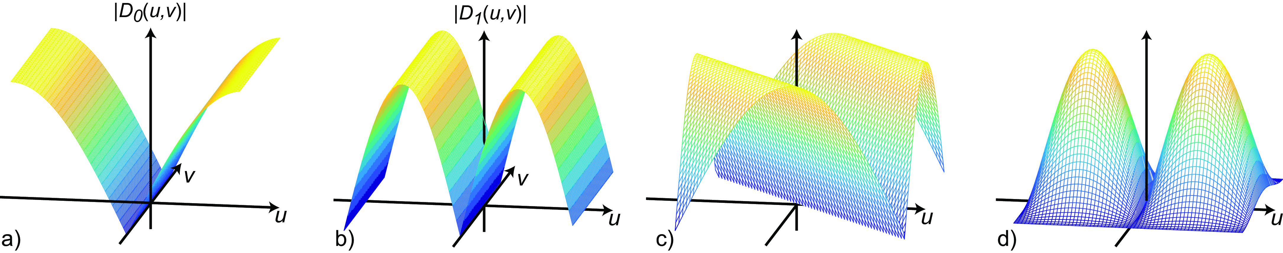
Figure 18.14 compares the DFT of the four types of approximations of the derivatives that we have discussed. These operators are still very popular. (Sobel) has the best tolerance to noise due to its band-pass nature. The kernel (d_0) is the one that provides the highest resolution in the output. Figure 18.15 shows the output of different derivative approximations to a simple input image containing a circle. In the next section, we will discuss how to use these derivatives to extract other interesting quantities.
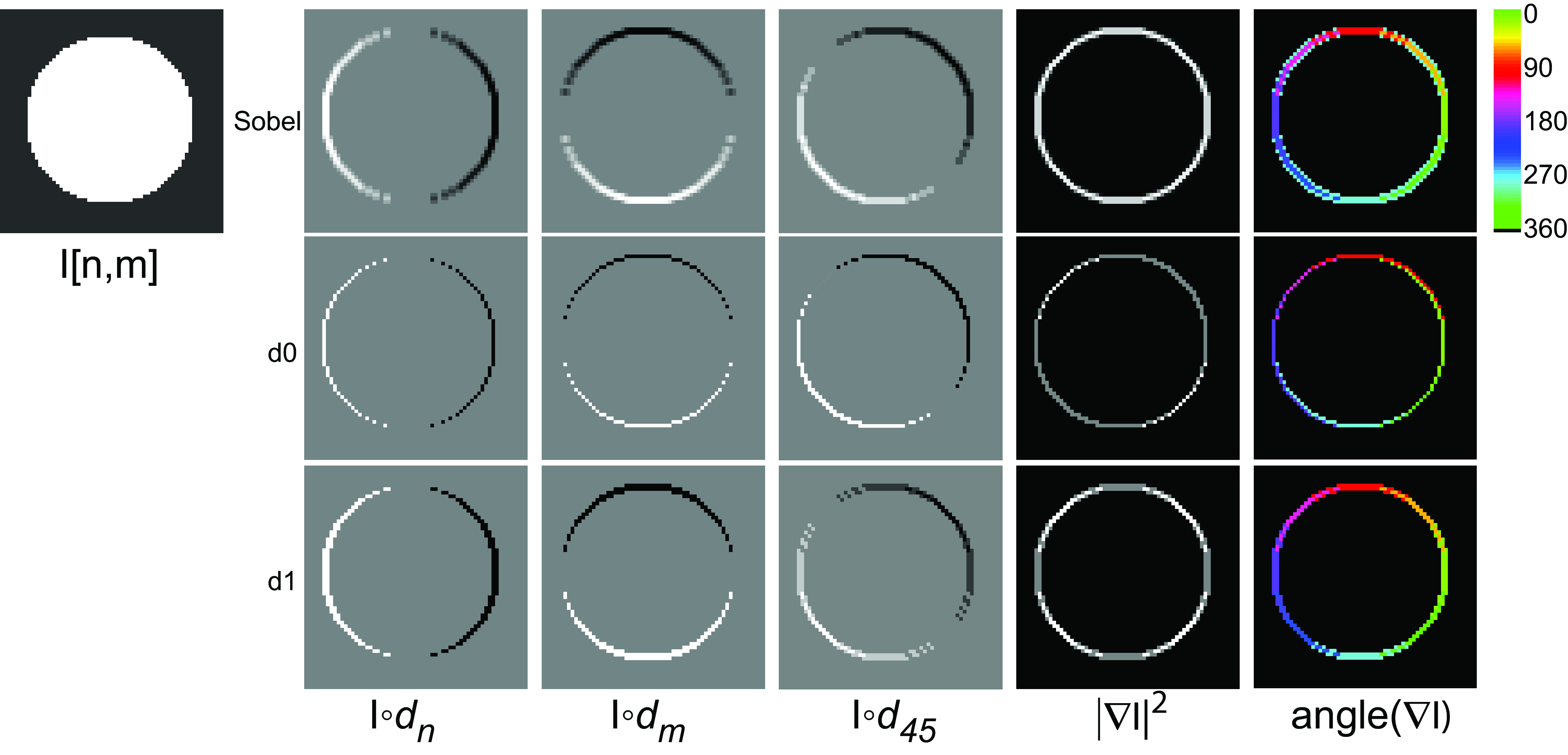
The angle is shown only where the magnitude is \(>0\). The derivative output along 45 degrees is obtained as a linear combination of the derivatives outputs along \(n\) and \(m\). Check the differences among the different kernels. The Sobel operator gives the most rotationally invariant gradient magnitude, but it is blurrier.
18.8 Image Gradient and Directional Derivatives
As we saw in Chapter 2, an important image representation is given by the image gradient. From the image derivatives, we can also define the image gradient as the vector: \[ \nabla \ell (x,y) = \left( \frac{\partial \ell(x,y)}{\partial x}, \frac{\partial \ell(x,y)}{\partial y} \right) \] For each pixel, the output is a 2D vector. In the case of using Gaussian derivatives, we can write: \[ \nabla \ell \circ g = \nabla g \circ \ell = \left( g_x(x,y), g_y(x,y) \right) \circ \ell \]
Although we have mostly computed derivatives along the \(x\) and \(y\) variables, we can obtain the derivative in any orientation as a linear combination of the two derivatives along the main axes. With \({\bf t}=\left( \cos (\theta), \sin(\theta) \right)\), we can write the directional derivative along the vector \({\bf t}\) as: \[ \frac{\partial \ell (x,y)}{\partial {\bf t}} = \nabla \ell \cdot {\bf t} = \cos(\theta) \frac{\partial \ell}{\partial x} + \sin(\theta) \frac{\partial \ell}{\partial y} \]
In the Gaussian case: \[ \begin{split} \frac{\partial \ell}{\partial {\bf t}} \circ g & = \left( \cos(\theta) g_x(x,y) + \sin(\theta) g_y(x,y) \right) \circ \ell \\ & = \left( \nabla g \cdot {\bf t} \right) \circ \ell \\ & = g_{\theta} (x,y) \circ \ell(x,y) \end{split} \tag{18.4}\]
with \(g_{\theta} (x,y) = \cos(\theta) g_x(x,y) + \sin(\theta) g_y(x,y)\). However, to compute the derivative along any arbitrary angle \(\theta\) does not require doing new convolutions. Instead, we can compute any derivative as a linear combination of the output of convolving the image with \(g_x(x,y)\) and \(g_y(x,y)\): \[ \frac{\partial \ell}{\partial {\bf t}} \circ g = \cos(\theta) g_x(x,y) \circ \ell + \sin(\theta) g_y(x,y) \circ \ell(x,y) \]
When using discrete convolutional kernels \(d_n\left[n,m\right]\) and \(d_m\left[n,m\right]\) to approximate the derivatives along \(n\) and \(m\), it can be written as: \[ \nabla \ell = \left( d_n\left[n,m\right], d_m\left[n,m\right] \right) \circ \ell \left[n,m\right] \] and \[ \frac{\partial \ell}{\partial {\bf t}} \circ g = d_{\theta} \left[n,m\right] \circ \ell \left[n,m\right] \]
with \(d_{\theta} \left[n,m\right] = \cos(\theta) d_n\left[n,m\right] + \sin(\theta) d_m\left[n,m\right]\). We expect that the linear combination of these two kernels should approximate the derivative along the direction \(\theta\). The quality of this approximation will vary for the different kernels we have seen in the previous sections.
18.9 Image Laplacian
The Laplacian filter was made popular by Marr and Hildreth in 1980 [6] in the search for operators that locate the boundaries between objects. The Laplacian is a common operator from differential geometry to measure the divergence of the gradient and it appears frequently in modeling fields in physics. The Laplacian also has applications in graph theory and in spectral methods for image segmentation [7].
One example of application of the Laplacian is in the paper Can One Hear the Shape of a Drum [8], where the Laplacian is used for modeling vibrations in a drum and the sounds it produces as a function of its shape.
The Laplacian operator is defined as the sum of the second order partial derivatives of a function:
\[ \nabla^2 \ell = \frac{\partial^2 \ell}{\partial x^2} + \frac{\partial^2 \ell}{\partial y^2} \]
The Laplacian is more sensitive to noise than the first order derivative. Therefore, in the presence of noise, when computing the Laplacian operator on an image \(\ell(x,y)\), it is useful to smooth the output with a Gaussian kernel, \(g(x,y)\). We can write,
\[ \nabla^2 \ell \circ g = \nabla^2 g \circ \ell \]
Therefore, the same result can be obtained if we first compute the Laplacian of the Gaussian kernel, \(g(x,y)\) and then convolve it with the input image. The Laplacian of the Gaussian is
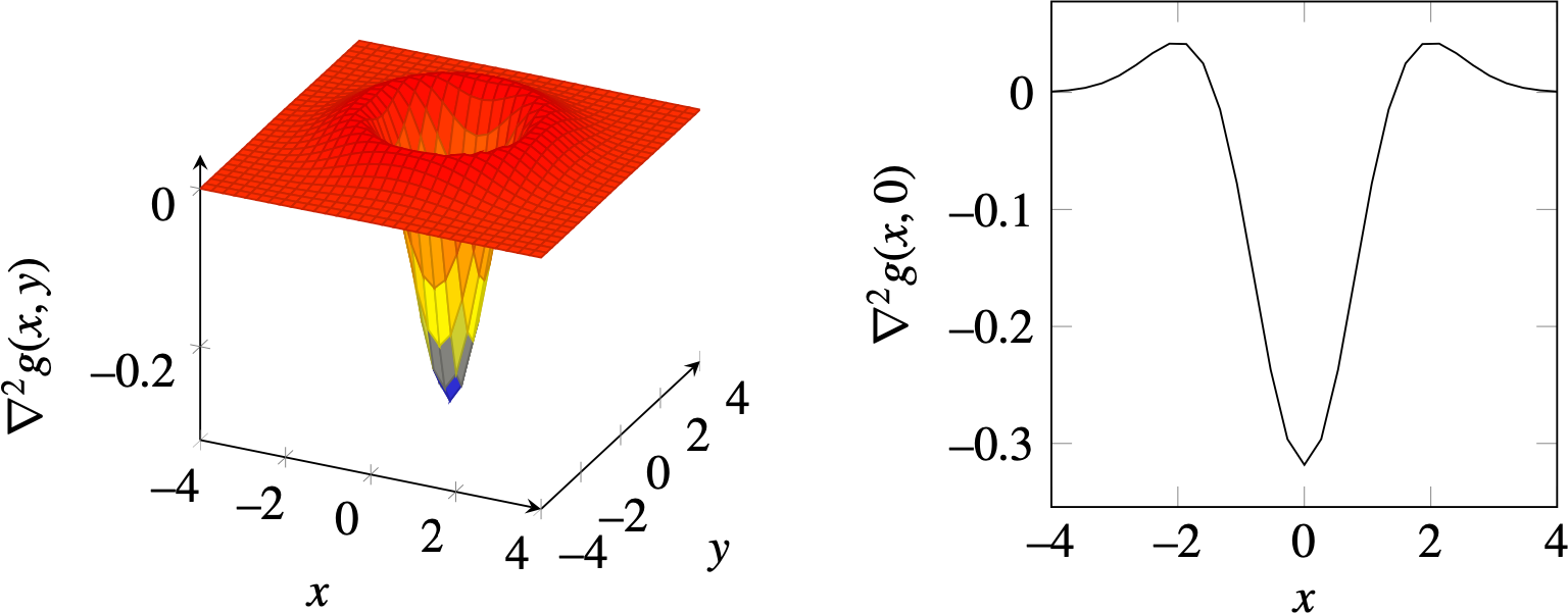
\[ \nabla^2 g = \frac{x^2 + y^2 -2\sigma^2}{\sigma^4} g(x,y) \]
The next plot (Figure 18.16) shows the Gaussian Laplacian (\(\sigma = 1\)). Due to its shape, the Laplacian is also called the inverted mexican hat wavelet.
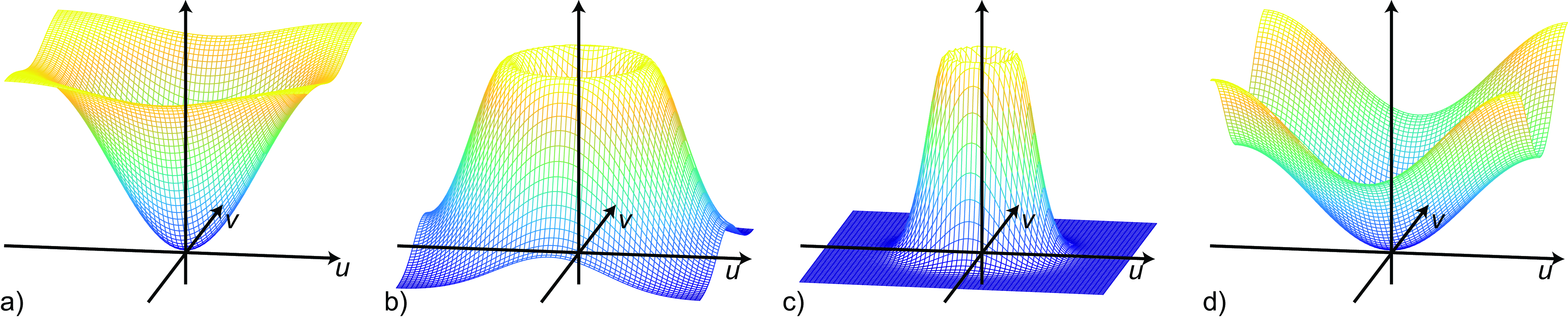
In the discrete domain, there are several approximations to the Laplacian filter. The simplest one consists in sampling the continuous Gaussian Laplacian in discrete locations. Figures Figure 18.17(a-c) show the DFT of the Gaussian Laplacian for three different values of \(\sigma\). For values \(\sigma > 1\), the resulting filter is band-pass, which is the expected behavior for the Gaussian Laplacian.
In one dimension, the Laplacian can be approximated by \([1,-2,1]\), which is the result of the convolution of two 2-tap discrete approximations of the derivative \([1,-1] \circ [1,-1]\). In two dimensions, the most popular approximation is the five-point formula, which consists of convolving the image with the kernel:
\[ \nabla_5^2 = \begin{bmatrix} 0 & 1 & 0 \\ 1 & -4 & 1\\ 0 & 1 & 0 \end{bmatrix} \tag{18.5}\]
It involves the central pixel and its four nearest neighbors. This is a sum-separable kernel: it corresponds to approximating the second-order derivative for each coordinate and summing the result (i.e., convolve the image with \([1,-2,1]\) and also with its transpose and summing the two outputs).
The Laplacian of the image, using the five-point formula, is:
\[ \begin{split} \nabla_5^2 \ell[n,m] = & - 4 \ell[n,m] \\ & + \ell[n+1,m] \\ & + \ell[n-1,m] \\ & + \ell[n,m+1] \\ & + \ell[n,m-1] \end{split} \]
Figure 18.18 compares the output of image derivatives and the Laplacian. Note that when summing two first-order derivatives along \(x\) and \(y\), what we obtain is a first-order derivative along the 45-degree angle. However, when summing up the two second-order derivatives, we obtain a rotationally invariant kernel, as shown in Figure 18.18(d).
The discrete approximation also provides a better intuition of how it works than its continuous counterpart. The Laplacian filter has a number of advantages with respect to the gradient:
- It is rotationally invariant. It is a linear operator that responds equally to edges in any orientation (this is only approximate in the discrete case).
- It measures curvature. If the image contains a linear trend the derivative will be non-zero despite having no boundaries, while the Laplacian will be zero.
- Edges can be located as the zero-crossings in the Laplacian output. However, this way of detecting edges is not very reliable.
- Zero crossings of an image form closed contours.
Figure 18.19 compares the output of the first-order derivative Figure 18.19 (b) and the Laplacian Figure 18.19 (d) on a simple 1D signal Figure 18.19 (a). The local maximum of the derivative output Figure 18.19 (c) and the zero crossings of the Laplacian output Figure 18.19 (e) are aligned with the transitions (boundaries) of the input signal Figure 18.19 (a).
Marr and Hildreth [6] used zero-crossings of the Laplacian output to compute edges, but this method is not used nowadays for edge detection. Instead, the Laplacian filter is widely used in a number of other image representations. It is used to build image pyramids (multiscale representations, see Chapter Chapter 23), and to detect points of interest in images (it is the basic operator used to detect keypoints to compute SIFT descriptors [2]).
18.10 A Simple Model of the Early Visual System
The Laplacian filter can also be used as a coarse approximation of the behavior of the early visual system. When looking at the magnitude of the DFT of the Laplacian with \(\sigma=1\) (Figure 18.17), the shape seems reminiscent of our subjective evaluation of our own visual sensitivity to spatial frequencies when we look at the Campbell and Robson chart (Figure 18.21). As the visual filter does not seem to cancel exactly the very low spatial frequencies as the Laplacian does, a better approximation is
\[ h = -\nabla^2 g + \lambda g \tag{18.6}\]
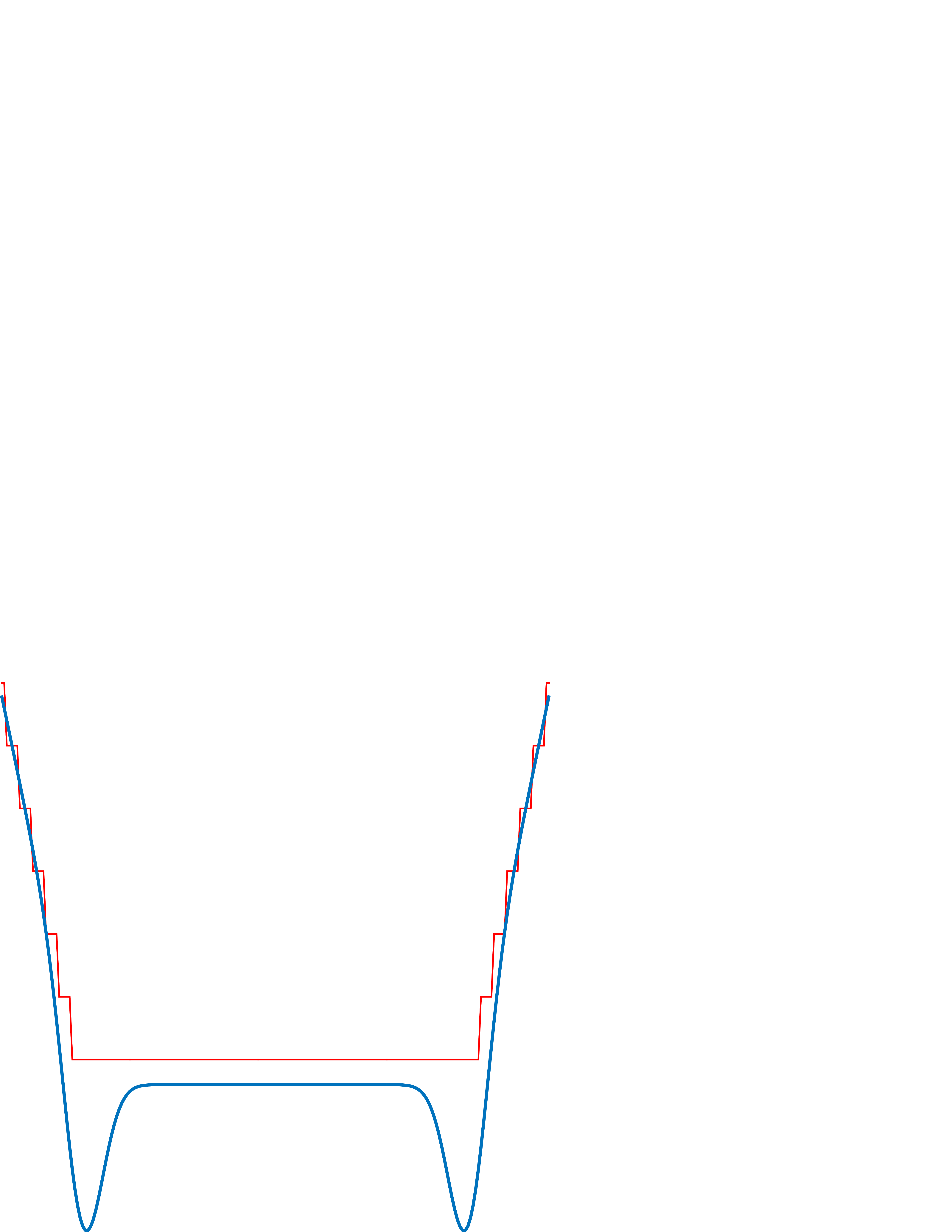
where the negative sign in front of the Laplacian helps to fit our perception better. The kernel \(h\) is the approximate impulse response of the human visual system, \(\lambda\) is a small constant that is equal to the DC gain of the visual filter (here we have set \(\lambda = 2\) and \(\sigma=5\)). This results in the profile shown in Figure 18.20.
The first thing worth pointing out is that the Fourier transform of the impulse response shown in Figure 18.20 has a shape that is qualitatively similar to the shape of the human contrast sensitivity function as discussed in Chapter 16. Here we show again the Campbell and Robson chart, together with a radial section of the Fourier transform of \(h\) from Equation 18.6:
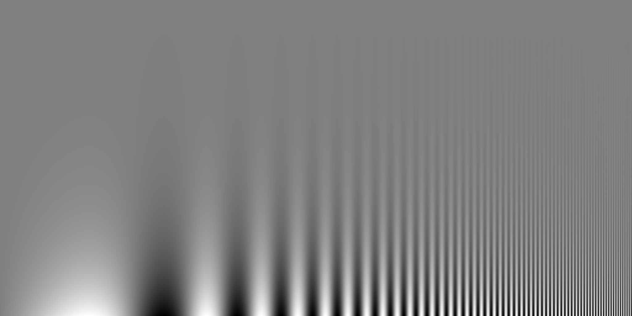

This particular form of impulse response explains some visual illusions as shown in Figure 18.22. This visual illusion is called the Vasarely visual illusion.


18.11 Sharpening Filter
One example of a simple but very useful filter is a sharpening filter. The goal of a sharpening filter is to transform an image so that it appears sharper (i.e., it contains more fine details). This can be achieved by amplifying the amplitude of the high-spatial frequency content of the image. We can achieve this with a combination of filters that we have already discussed in this section.
A simple way to design a sharpening filter is to de-emphasize the blurry components of an image. By the linearity of the convolution operator, we’re allowed to add and subtract kernels to make a new kernel that would give us the same filtered image as if we had added and subtracted the filtered outputs of each of the component kernels. For this example, we start with twice the original image (sharp plus blurred parts), then subtract away the blurred components of the image:
\[ \text{sharpening filter} = \begin{bmatrix} 0 & 0 & 0 \\ 0 & 2 & 0\\ 0 & 0 & 0 \end{bmatrix} - \frac{1}{16} \begin{bmatrix} 1 & 2 & 1 \\ 2 & 4 & 2\\ 1 & 2 & 1 \end{bmatrix} \tag{18.7}\]
Note that the DC gain of this sharpening filter is 1. That would leave one original image in there, plus an additional component of the sharp details. The perceptual result is that of a sharpened image (Figure 18.23). We can apply this filter successively in order to further enhance the image details. If too much sharpening is applied, we might end up enhancing noise and introducing image artifacts.


Note that the sharpening filter described here does not introduce new fine image details, it only enhances the ones already present in the image.
It is also interesting to note that this sharpening filter is very similar to the model of the early visual system that we described before.
18.12 Retinex
How do you tell gray from white? This might seem like a simple question, but one remarkable aspect of vision is that perception of the simplest quantity might be far from trivial. As a final example to illustrate the power of using image derivatives as an image representation, we will discuss here a partial answer to this question.
To understand that answering this question is not trivial, let’s consider the structure of light that reaches the eye, which is the input upon which our visual system will try to differentiate black from white. The amount of light that reaches the eye from a painted piece of paper is the result of two quantities: the amount of light reaching the piece of paper, and the reflectance of the surface (what fraction of the light is reflected back into space and what fraction is absorbed by the material).
If two patches receive the same amount of light, then we will perceive as being darker the patch that reflects less light. But what happens if we change the amount of light that reaches the scene? If we increase the amount of light projected on top of the dark patch, what will be seen now? What will happen if we have two patches on the same scene, each of them receiving different amounts of light? How does the visual system decide what white is and how does it deal with changes in the amount of light illuminating the scene? The visual system is constantly trying to estimate what the incident illumination is and what are the actual reflectances of the surfaces present in the scene.
If our goal is to estimate the shade of gray of a piece of painted paper, then the quantity that we care about is the reflectance of the surface. But, what happens if we see two patches of unknown reflectance, and each is illuminated with two different light sources of unknown identity? How does the visual system manage to infer what the illumination and reflectances are?

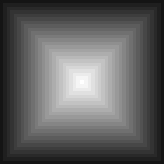
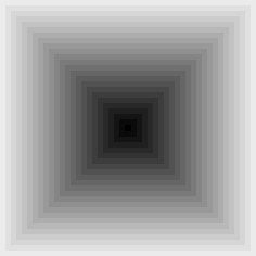
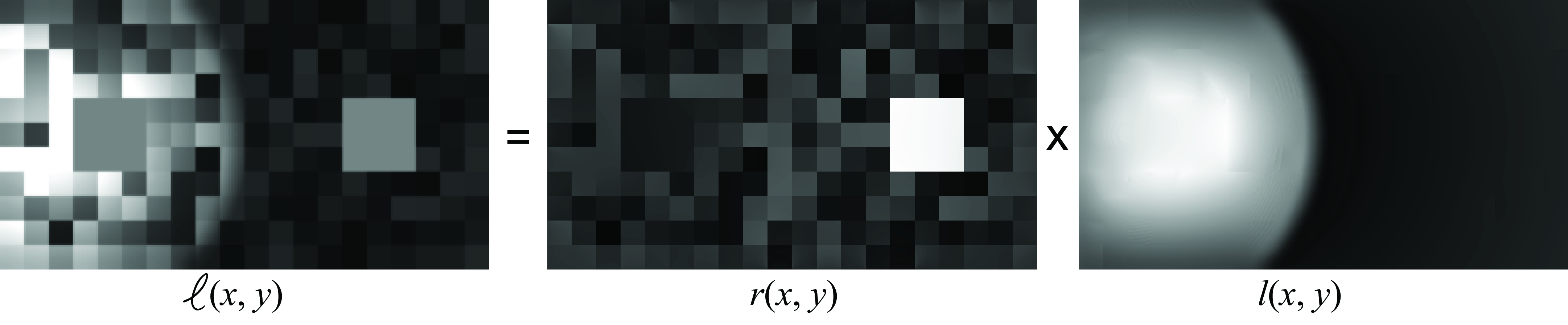
Visual illusions are a way of getting to feel how our own visual system processes images. To experience how this estimation process works, let’s start by considering a very simple image as shown in Figure 18.24. This image shows a very simple scene formed by a surface with a set of squares of different gray levels illuminated by a light spot oriented toward the left. Our visual system tries to estimate the two quantities: the reflectance of each square and the illumination intensity reaching each pixel.
Let’s think of the image formation process. The surface is made of patches of different reflectances \(r(x,y) \in (0,1)\). Each location receives an illumination \(l(x,y)\). The observed brightness is the product:
\[ \ell(x,y) = r(x,y) \times l(x,y) \]
Despite what reaches the eye is the signal \(\ell(x,y)\), our perception is not the value of \(\ell(x,y)\). In fact, the squares 1 and 2 in Figure 18.24 have the exact same values of intensity, but we see them differently, which is generally explained by saying that we discount (at least partially) the effects of the illumination, \(l(x,y)\).
The Retinex algorithm, by Land and McCann [9], is based on modeling images as if they were part of a Mondrian world (images that look like the paintings of Piet Mondrian). One example of a color Mondrian is:

But how can we estimate \(r(x,y)\) and \(l(x,y)\) by only observing \(\ell(x,y)\)? One of the first solutions to this problem was the Retinex algorithm proposed by Land and McCann [9]. Land and McCann observed that it is possible to extract \(r\) and \(l\) from \(\ell\) if one takes into account some constraints about the expected nature of the images \(r\) and \(l\). Land and McCann noted that if one considers two adjacent pixels inside one of the patches of uniform reflectance, the difference between the two pixel values will be very small as the illumination, even if it is nonuniform, will only produce a small change in the brightness of the two pixels. However, if the two adjacent pixels are on the boundary between two patches of different reflectances, then the intensities of these two pixels will be very different.
The Retinex algorithm works by first extracting \(x\) and \(y\) spatial derivatives of the image \(\ell(x,y)\) and then thresholding the gradients. First, we transform the product into a sum using the \(\log\):
\[ \log \ell(x,y) = \log r(x,y) + \log l(x,y) \]
Taking derivatives along \(x\) and \(y\) is now simple:
\[ \frac{\partial \log \ell(x,y)}{\partial x} = \frac{\partial \log r(x,y)}{\partial x} + \frac{\partial \log l(x,y)}{\partial x} \]
And the same thing is done for the derivative along \(y\).
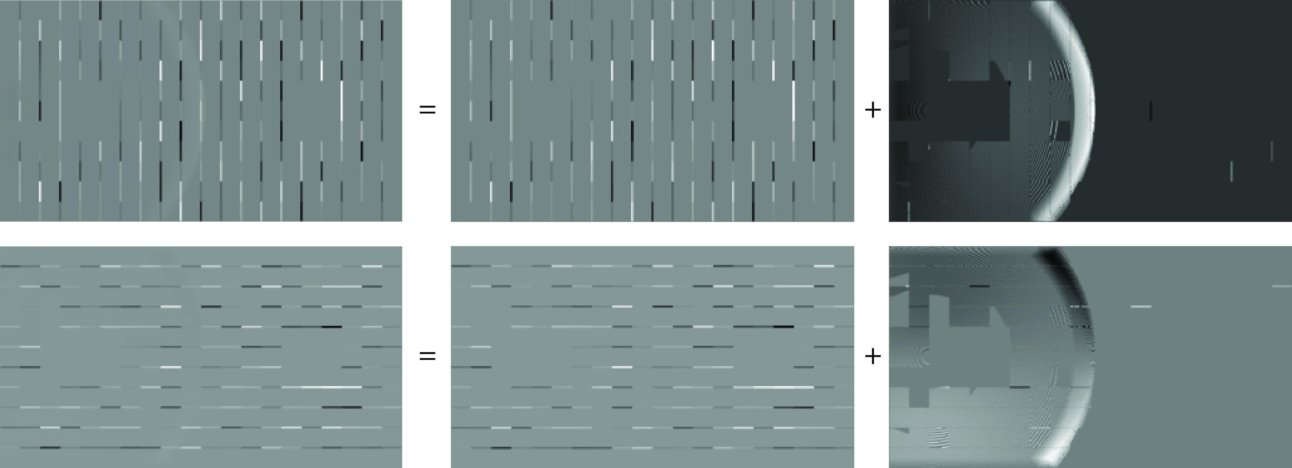
Any derivative larger than the threshold is assigned to the derivative of the reflectance image \(r(x,y)\), and the ones smaller than a threshold are assigned to the illumination image \(l(x,y)\):
\[ \frac{\partial \log r(x,y)}{\partial x} = \begin{cases} \frac{\partial \log \ell(x,y)}{\partial x} & \text{if} ~ \left| \frac{\partial \log \ell(x,y)}{\partial x} \right|>T\\ 0 & \text{otherwise} \end{cases} \]
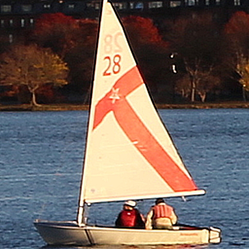
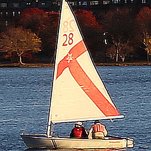
Figure 18.25 shows how the image derivatives are decomposed into reflectance and illumination changes.
Then, the image \(\log r(x,y)\) is obtained by integrating the gradients, as shown in Section 18.4, and exponentiating the result. Finally, the illumination can be obtained as \(l(x,y) = \ell(x,y)/r(x,y)\). The results are shown in Figure 18.26.
Note that the illumination derivatives have much lower magnitude than the reflectance derivatives; however, they extend over much larger spatial regions, which means that once they are integrated, changes in brightness due to nonuniform illumination might be larger than changes due to variations in reflectance values.
Despite the simplicity of this approach, it works remarkably well with images like the ones shown in Figure 18.24 and also with a number of real images. However, the algorithm is limited and it is easy to make it fail in situations where the visual system works, as we will see later in more depth.
The Retinex algorithm works by making assumptions about the structure of the images it tries to separate. The underlying assumption is that the illumination image, \(l(x,y)\), varies smoothly and the reflectance image, \(r(x,y)\), is composed of uniform regions separated by sharp boundaries. These assumptions are very restrictive and will limit the domain of applicability of such an approach. Understanding the structure of images in order to build models such as Retinex has been the focus of a large amount of research. This chapter will introduce some of the most important image models.
The recovered brightness is stronger than what we perceive. There are a number of reasons that weaken the perceived brightness. The effect is bigger if the display occupies the entire visual field. Right now the picture appears in the context of the page, which also affects our perception of the illumination. Also, the two larger squares do not seem to group well with the rest of the display, as if they were floating in a different plane. And finally, for such a simple display, the visual system does not fully separate the perception of both components.
Decomposing an image into different physical causes is known as intrinsic images decomposition. The intrinsic image decomposition, proposed by Barrow and Tenenbaum [10], aims to recover intrinsic scene characteristics from images, such as occlusions, depth, surface normals, shading, reflectance, reflections, and so on.
18.13 Concluding Remarks
In this chapter we have covered a very powerful image representation: image derivatives (first order, second order, and the Laplacian) and their discrete approximations. Despite the simplicity of this representation, we have seen that it can be used in a number of applications such as image inpaining, separation of illumination and reflectance, and it can be used to explain simple visual illusions. It is not surprising that similar filters like the ones we have seen in this chapter emerge in convolutional neural networks when trained to solve visual tasks.