15 Linear Image Filtering
15.1 Introduction
We want to build a vision system that operates in the real world. One such system is the human visual system. Although much remains to be understood about how our visual system processes images, we have a fairly good idea of what happens at the initial stages of visual processing, and it will turn out to be similar to some of the filtering we discuss in this chapter. While we’re inspired by the biology, here we describe some mathematically simple processing that will help us to parse an image into useful tokens, or low-level features that will be useful later to construct visual interpretations.
We’d like for our processing to enhance image structures of use for subsequent interpretation, and to remove variability within the image that makes more difficult comparisons with previously learned visual signals. Let’s proceed by invoking the simplest mathematical processing we can think of: a linear filter. Linear filters as computing structures for vision have received a lot of attention because of their surprising success in modeling some aspect of the processing carried out by early visual areas such as the retina, the lateral geniculate nucleus (LGN) and primary visual cortex (V1) [1]. In this chapter we will see how far it takes us toward these goals.
For a deeper understanding there are many books [2] devoted to signal processing, providing essential tools for any computer vision scientist. In this chapter we will present signal processing tools from a computer vision and image processing perspective.
15.2 Signals and Images
A signal is a measurement of some physical quantity (light, sound, height, temperature, etc.) as a function of another independent quantity (time, space, wavelength, etc.). A system is a process/function that transforms a signal into another.
15.2.1 Continuous and Discrete Signals
Although most of the signals that exist in nature are infinite continuous signals, when we introduce them into a computer they are sampled and transformed into a finite sequence of numbers, also called a discrete signal.
Sampling is the process of transforming a continuous signal into a discrete one and will be studied in detail in Chapter 20.
If we consider the light that reaches one camera photo sensor, we could write it as a one dimensional function of time, \(\ell(t)\), where \(\ell(t)\) denotes the incident \(\ell\)ight at time \(t\), and \(t\) is a continuous variable that can take on any real value. The signal \(\ell(t)\) is then sampled in time (as is done in a video) by the camera where the values are only captured at discrete times (e.g., 30 times per second). In that case, the signal \(\ell\) will be defined only on discrete time instants and we will write the sequence of measured values as: \(\ell\left[ n \right]\), where \(n\) can only take on integer values. The relationship between the discrete and the continuous signals is given by the sampling equation: \[\ell\left[n\right] = \ell\left(n~\Delta T \right)\] where \(\Delta T\)is the sampling period. For instance, \(\Delta T = 1/30\) s in the case of sampling the signal 30 times per second.
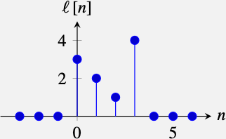
As is common in signal processing, we will use parenthesis to indicate continuous variables and brackets to denote discrete variables. For instance, if we sample the signal shown in Figure 15.1 (a) once every second (\(\Delta T = 1\) s) we get the discrete signal shown in Figure 15.1 (b).
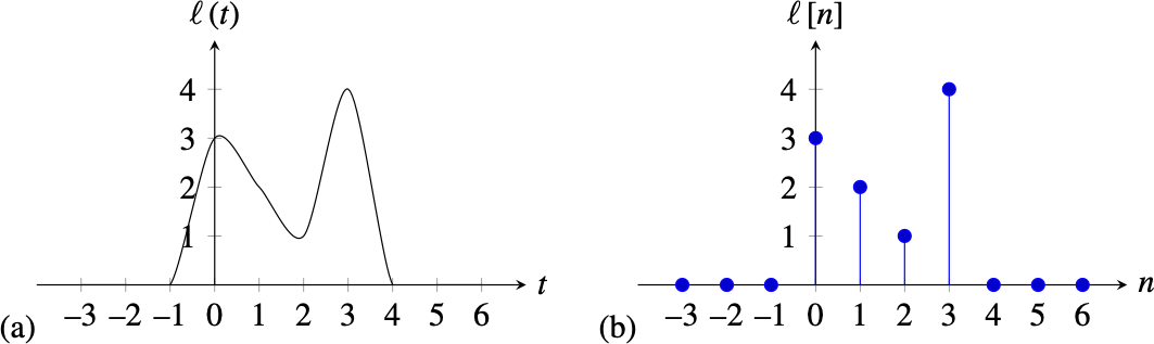
The signal in Figure 15.1 (b) is a function that takes on the values \(\ell\left[0\right] = 3\), \(\ell\left[1\right] = 2\), \(\ell\left[2\right] = 1\) and \(\ell\left[3\right] = 4\) and all other values are zero, \(\ell\left[n\right] = 0\). In most of the book we will work with discrete signals. In many cases it will be convenient to write discrete signals as vectors. Using vector notation we will write the previous signal, in the interval \(n \in \left[0,6 \right],\) as a column vector \(\boldsymbol\ell= \left[3, 2, 1, 4, 0, 0, 0\right]^T\), where \(T\) denotes transpose.
15.2.2 Images
An image is a two dimensional array of values: \(\boldsymbol\ell\in \mathbb{R}^{M \times N}\), where \(N\) is the image width and \(M\) is the image height. A grayscale image is then just an array of numbers such as the following (in this example, intensity values are scaled between 0 and 256):
\[\begin{array}{cc} \boldsymbol\ell= & \left[ \begin{smallmatrix} 160 & 175 & 171 & 168 & 168 & 172 & 164 & 158 & 167 & 173 & 167 & 163 & 162 & 164 & 160 & 159 & 163 & 162\\ 149 & 164 & 172 & 175 & 178 & 179 & 176 & 118 & 97 & 168 & 175 & 171 & 169 & 175 & 176 & 177 & 165 & 152\\ 161 & 166 & 182 & 171 & 170 & 177 & 175 & 116 & 109 & 169 & 177 & 173 & 168 & 175 & 175 & 159 & 153 & 123\\ 171 & 174 & 177 & 175 & 167 & 161 & 157 & 138 & 103 & 112 & 157 & 164 & 159 & 160 & 165 & 169 & 148 & 144\\ 163 & 163 & 162 & 165 & 167 & 164 & 178 & 167 & 77 & 55 & 134 & 170 & 167 & 162 & 164 & 175 & 168 & 160\\ 173 & 164 & 158 & 165 & 180 & 180 & 150 & 89 & 61 & 34 & 137 & 186 & 186 & 182 & 175 & 165 & 160 & 164\\ 152 & 155 & 146 & 147 & 169 & 180 & 163 & 51 & 24 & 32 & 119 & 163 & 175 & 182 & 181 & 162 & 148 & 153\\ 134 & 135 & 147 & 149 & 150 & 147 & 148 & 62 & 36 & 46 & 114 & 157 & 163 & 167 & 169 & 163 & 146 & 147\\ 135 & 132 & 131 & 125 & 115 & 129 & 132 & 74 & 54 & 41 & 104 & 156 & 152 & 156 & 164 & 156 & 141 & 144\\ 151 & 155 & 151 & 145 & 144 & 149 & 143 & 71 & 31 & 29 & 129 & 164 & 157 & 155 & 159 & 158 & 156 & 148\\ 172 & 174 & 178 & 177 & 177 & 181 & 174 & 54 & 21 & 29 & 136 & 190 & 180 & 179 & 176 & 184 & 187 & 182\\ 177 & 178 & 176 & 173 & 174 & 180 & 150 & 27 & 101 & 94 & 74 & 189 & 188 & 186 & 183 & 186 & 188 & 187\\ 160 & 160 & 163 & 163 & 161 & 167 & 100 & 45 & 169 & 166 & 59 & 136 & 184 & 176 & 175 & 177 & 185 & 186\\ 147 & 150 & 153 & 155 & 160 & 155 & 56 & 111 & 182 & 180 & 104 & 84 & 168 & 172 & 171 & 164 & 168 & 167\\ 184 & 182 & 178 & 175 & 179 & 133 & 86 & 191 & 201 & 204 & 191 & 79 & 172 & 220 & 217 & 205 & 209 & 200\\ 184 & 187 & 192 & 182 & 124 & 32 & 109 & 168 & 171 & 167 & 163 & 51 & 105 & 203 & 209 & 203 & 210 & 205\\ 191 & 198 & 203 & 197 & 175 & 149 & 169 & 189 & 190 & 173 & 160 & 145 & 156 & 202 & 199 & 201 & 205 & 202\\ 153 & 149 & 153 & 155 & 173 & 182 & 179 & 177 & 182 & 177 & 182 & 185 & 179 & 177 & 167 & 176 & 182 & 180 \end{smallmatrix}\right] \end{array}\]
This matrix represents an image of size \(18 \times 18\) pixels as encoded in a computer. Can you guess what object appears in the array? The goal of a computer vision system is to reorganize this array of numbers into a meaningful representation of the scene depicted in the image. The next image shows the same array of values but visualized as gray levels.
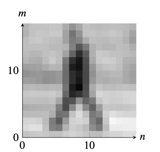
When we want to make explicit the location of a pixel we will write \(\ell\left[n, m \right]\), where \(n \in \left[0,N-1 \right]\) and \(m \in \left[0,M-1 \right]\) are the indices for the horizontal and vertical dimensions, respectively. Each value in the array indicates the intensity of the image in that location. For color images we will have three channels, one for each color.
Although images are discrete signals, in some cases it is useful to work on the continuous domain as it simplifies the derivation of analytical solutions. This was the case in the previous chapter where we used the image gradient in the continuous domain and then approximated it in the discrete space domain. In those cases we will write images as \(\ell(x,y)\) and video sequences as \(\ell(x,y,t)\).
15.2.3 Properties of a Signal
Here are some important quantities that are useful to characterize signals. As most signals represent physical quantities, a lot of the terminology used to describe them is borrowed from physics.
Both continuous and discrete signals can be classified according to its extend. Infinite length signals are signals that extend over the entire support \(\ell\left[n \right]\) for \(n \in (-\infty, \infty)\). Finite length signals have non-zero values on a compact time interval and they are zero outside, i.e. \(\ell\left[n \right] = 0\) for \(n \notin S\) where \(S\) is a finite length interval. A signal \(\ell\left[n \right]\) is periodic if there is a value \(N\) such that \(\ell\left[n \right] = \ell\left[n + k N\right]\) for all \(n\) and \(k\). A periodic signal is an infinite length signal. An important quantity is the mean value of a signal often called the DC value.
DC means direct current and it comes from electrical engineering. Although most signals have nothing to do with currents, the term DC is still commonly used.
In the case of an image, the DC component is the average intensity of the image. For a finite signal of length \(N\) (or a periodic signal), the DC value is \[\mu = \frac{1}{N} \sum_{n=0}^{N-1} \ell\left[n\right]\] If the signal is infinite, the average value is \[\mu = \lim_{N \xrightarrow{} \infty} \frac{1}{2N+1} \sum_{n=-N}^{N} \ell\left[n\right]\]
Another important quantity to characterize a signal is its energy. Following the same analogy with physics, the energy of a signal is defined as the sum of squared magnitude values: \[E = \sum_{n = -\infty}^{\infty} \left| \ell\left[n\right] \right| ^2\]
Signal energy and general energy are equivalent up to a normalization constant. For instance, the energy dissipated by a resistance \(R\) with voltage \(v(t)\) is \[\begin{equation} E = \frac{1}{R} \int_{-\infty}^{\infty} v(t) ^2 dt \end{equation}\]
Signal are further classified as finite energy and infinite energy signals. Finite length signals are finite energy and periodic signals are infinite energy signals when measuring the energy in the whole time axis.
If we want to compare two signals, we can use the squared Euclidean distance (squared L2 norm) between them: \[D^2 = \frac{1}{N} \sum_{n=0}^{N-1} \left| \ell_1 \left[n\right] - \ell_2 \left[n\right] \right| ^2\] However, the euclidean distance (L2) is a poor metric when we are interested in comparing the content of the two images and the building better metrics is an important area of research. Sometimes, the metric is L2 but in a different representation space than pixel values. We will talk about this more later in the book.
The same definitions apply also to continuous signals, where all the equations are analogous by replacing the sums with integrals. For instance, in the case of the energy of a continuous signal, we can write \(E = \int_{-\infty}^{\infty} \left| \ell\left( t \right) \right|^2 dt\), which assumes that the integral is finite. Most natural signals will have infinite energy.
15.3 Systems
The kind of systems that we will study here take a signal, \(\boldsymbol\ell_{\texttt{in}}\), as input, perform some computation, \(f\), and output another signal, \(\boldsymbol\ell_{\texttt{out}}= f(\boldsymbol\ell_{\texttt{in}})\).
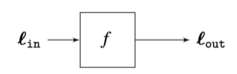
This transformation is very general and it can do all sorts of complex things: it could detect edges in images, recognize objects, detect motion in sequences, or apply aesthetic transformations to a picture. The function \(f\) could be specified as a mathematical operation or as an algorithm. As a consequence, it is very difficult to find a simple way of characterizing what the function \(f\) does. In the next section we will study a simple class of functions \(f\) that allow for a simple analytical characterization: linear systems.
15.3.1 Linear Systems
Linear systems represent a very small portion of all the possible systems one could implement, but we will see that they are capable of creating very interesting image transformations. A function \(f\) is linear if it satisfies the following two properties:
\[\begin{aligned} f\left( \boldsymbol\ell_1+\boldsymbol\ell_2 \right) &=& f(\boldsymbol\ell_1)+ f(\boldsymbol\ell_2) \\ \nonumber f(a\boldsymbol\ell) &=& af(\boldsymbol\ell) ~~\text{~for any scalar~} a \end{aligned}\]
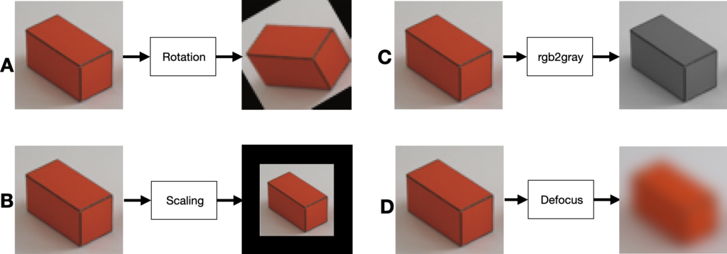
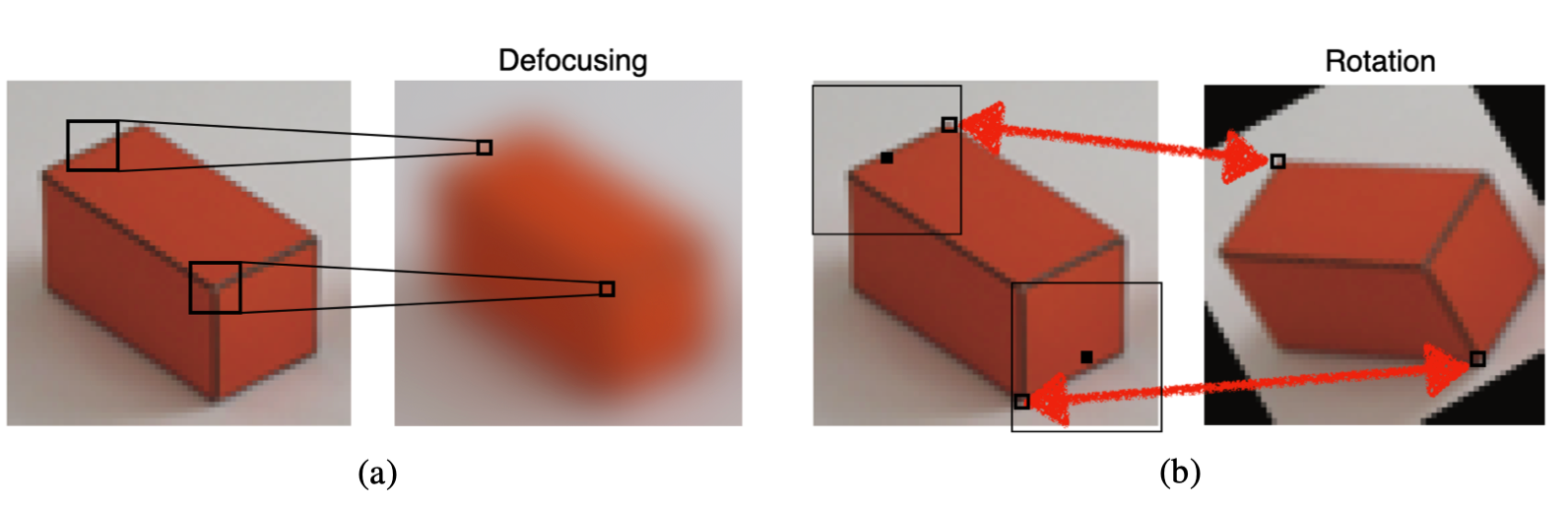
Although the previous properties might seem simple, it is easy to get confused on when an operation can be or not represented by a linear function. Let’s first check your intuition about what operations are linear and which ones are not. Which ones of the image transformations shown in Figure 15.3 can be written as linear systems?
To make things more concrete, lets assume the input is a 1D signal with length \(N\) that we will write as \(\ell_{\texttt{in}}\left[n \right]\), and the output is another 1D signal with length \(M\) that we will write as \(\ell_{\texttt{out}}\left[n \right]\). Most of the times we will work with input and output pairs with the same length \(M=N\). A linear system, in its most general form, can be written as follows: \[\ell_{\texttt{out}}\left[n \right] = \sum_{k=0}^{N-1} h \left[n,k\right] \ell_{\texttt{in}}\left[k \right] ~~~ for ~~~ n \in \left[0, M-1 \right] \tag{15.1}\] where each output value \(\ell_{\texttt{out}}\left[n \right]\) is a linear combination of values of the input signal \(\ell_{\texttt{in}}\left[n \right]\) with weights \(h \left[n,k\right]\). The value \(h \left[n,k\right]\) is the weight applied to the input sample \(\ell_{\texttt{in}}\left[k \right]\) to compute the output sample \(\ell_{\texttt{out}}\left[n \right]\). To help visualizing the operation performed by the linear filter it is useful to write it in matrix form: \[\begin{bmatrix}\ell_{\texttt{out}}\left[ 0 \right] \\ \ell_{\texttt{out}}\left[ 1 \right] \\ \vdots \\ \ell_{\texttt{out}}\left[ n \right] \\ \vdots \\ \ell_{\texttt{out}}\left[ M-1 \right] \end{bmatrix} = \begin{bmatrix} h\left[0,0\right] ~&~ h\left[0,1\right] ~&~ ... ~&~ h\left[0,N-1\right] \\ h\left[1,0\right] ~&~ h\left[1,1\right] ~&~ ... ~&~ h\left[1,N-1\right] \\ \vdots ~&~ \vdots ~&~ \vdots ~&~ \vdots \\ \vdots ~&~ \vdots ~&~ h \left[n,k\right] ~&~ \vdots \\ \vdots ~&~ \vdots ~&~ \vdots ~&~ \vdots \\ h\left[M-1,0\right] ~&~ h\left[M-1,1\right] ~&~ ... ~&~ h\left[M-1,N-1\right] \end{bmatrix} ~ \begin{bmatrix} \ell_{\texttt{in}}\left[0\right] \\ \ell_{\texttt{in}}\left[1\right] \\ \vdots \\ \ell_{\texttt{in}}\left[k\right] \\ \vdots \\ \ell_{\texttt{in}}\left[N-1\right] \end{bmatrix}\] which we will write in short form as \(\boldsymbol\ell_{\texttt{out}}= \mathbf{H} \boldsymbol\ell_{\texttt{in}}\). The matrix \(\mathbf{H}\) has size \(M \times N\). We will use the matrix formulation many times in this book.
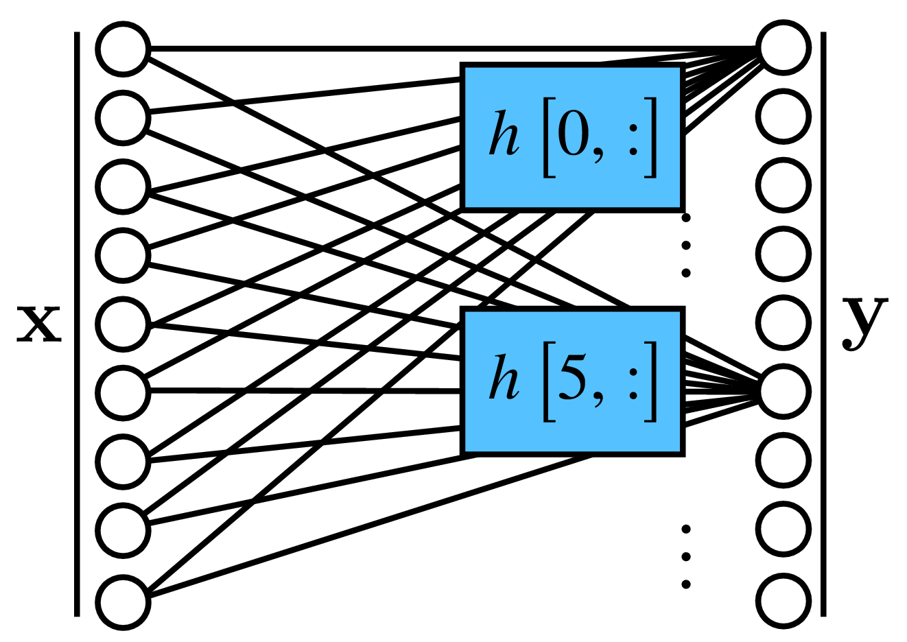
A linear function can also be drawn as a fully connected layer in a neural network, with weights \(\mathbf{W} = \mathbf{H}\), where the output unit \(i\), \(\ell_{\texttt{out}}\left[i \right]\), is a linear combination of the input signal \(\boldsymbol\ell_{\texttt{in}}\) with weights given by the row vectors of \(\mathbf{H}\). Graphically it looks like this:
In two dimensions the equations are analogous. Each pixel of the output image, \(\ell_{\texttt{out}}\left[n,m\right]\), is computed as a linear combination of pixels of the input image, \(\ell_{\texttt{in}}\left[n, m\right]\): \[\ell_{\texttt{out}}\left[n,m \right] = \sum_{k=0}^{M-1} \sum_{l=0}^{N-1} h \left[n,m,k,l \right] \ell_{\texttt{in}}\left[k,l \right] \tag{15.2}\] By writing the images as column vectors, concatenating all the image columns into a long vector, we can also write the previous equation using matrices and vectors: \(\boldsymbol\ell_{\texttt{out}}= \mathbf{H} \boldsymbol\ell_{\texttt{in}}\).
15.3.2 Linear Translation Invariant Systems
Linear systems are still too general for us. So let’s consider an even smaller family of systems: linear translation invariant (LTI) systems.
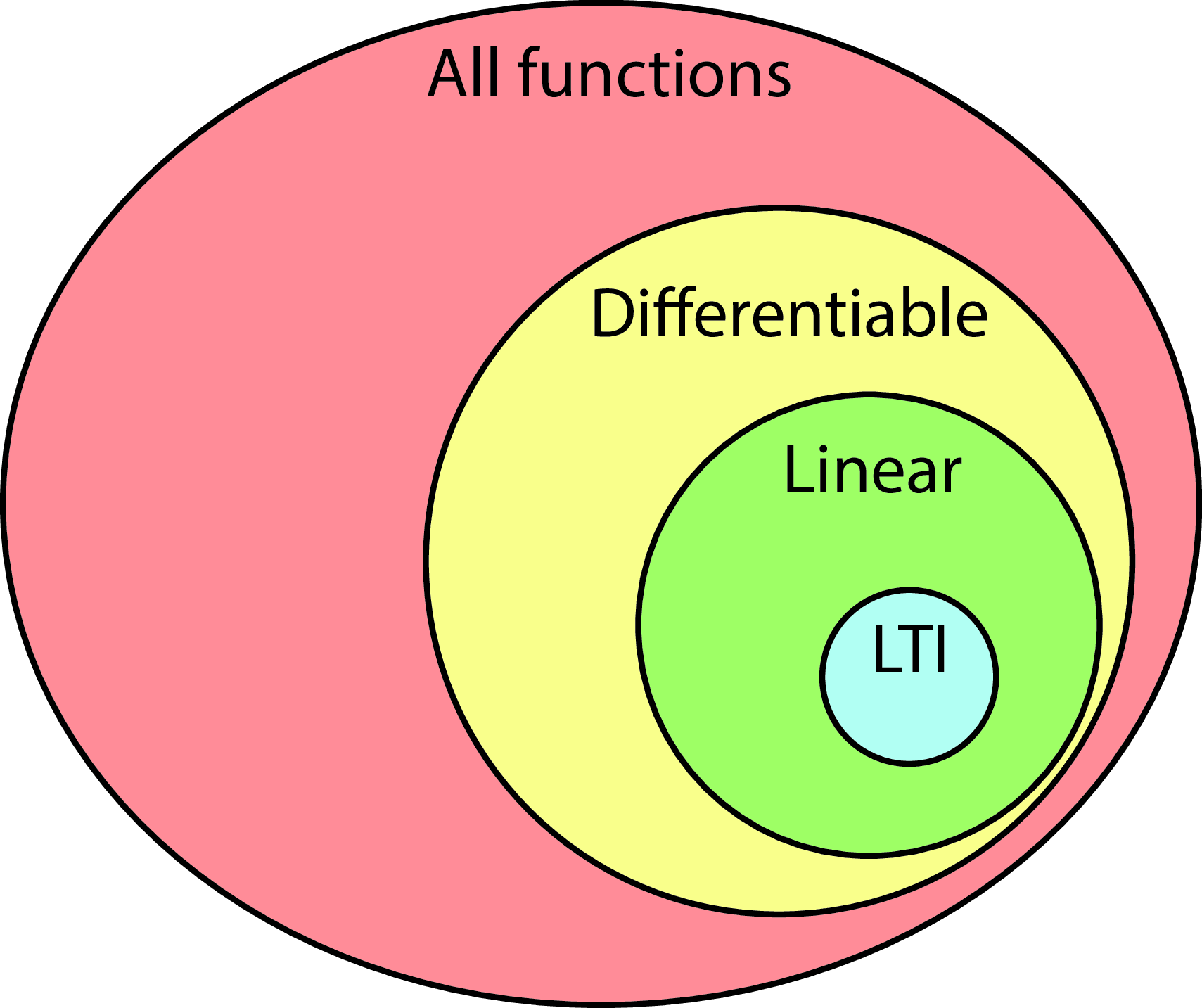
Translation invariant systems are motivated by the following observation: typically, we don’t know where within the image we expect to find any given item (Figure 15.5), so we often want to process the image in a spatially invariant manner, the same processing algorithm at every pixel.

An example of a translation invariant system is a function that takes as input an image and computes at each location a local average value of the pixels around in a window of \(5 \times 5\) pixels:
\[\ell_{\texttt{out}}\left[n,m \right] = \frac{1}{25} \sum_{k=-2}^{2} \sum_{l=-2}^{2} \ell_{\texttt{in}}\left[n+k,m+l \right]\]
A system is an LTI system if it is linear and when we translate the input signal by \(n_0, m_0\), then output is also translated by \(n_0, m_0\): \[\ell_{\texttt{out}}\left[ n - n_0, m-m_0 \right] = f \left( \ell_{\texttt{in}}\left[ n-n_0, m-m_0 \right] \right)\] for any \(n_0,m_0\). This property is called equivariant with respect to translation. Translation invariance and linearity impose a strong constraint on the form of equation (Equation 15.1).
In that case, the linear system becomes a convolution of the image data with some convolution kernel. This operation is very important and we devote the rest of this chapter to study its properties.
15.4 Convolution
The convolution, denoted \(\circ\), between a signal \(\ell_{\texttt{in}}\left[n \right]\) and the convolutional kernel \(h\left[n \right]\) is defined as follows: \[\ell_{\texttt{out}}\left[n\right] = h \left[n\right] \circ \ell_{\texttt{in}}\left[n\right] = \sum_{k=-\infty}^{\infty} h \left[n-k \right] \ell_{\texttt{in}}\left[k \right] \tag{15.3}\]
The convolution computes the output values as a linear weighted sum. The weight between the input sample \(\ell_{\texttt{in}}\left[k \right]\) and the output sample \(\ell_{\texttt{out}}\left[n\right]\) is a function \(h\left[n, k \right]\) that depends only on their relative position \(n-k\). Therefore, \(h\left[n, k \right]=h\left[n-k \right]\). If the signal \(\ell_{\texttt{in}}\left[n \right]\) has a finite length, \(N\), then the sum is only done in the interval \(k \in \left[0,N-1\right]\).
The convolution is related to the correlation operator. In the correlation, the weights are defined as \(h\left[n, k \right]=h\left[k-n \right]\). The convolution and the correlation use the same kernel but mirrored around the origin. The correlation is also translation invariant as we will discuss at the end of the chapter.
Most of the literature in neural networks calls convolution to the correlation operator. As the kernels are learned, the distinction is not important most of the time.
One important property of the convolution is that it is commutative: \(h\left[n\right] \circ \ell\left[n\right] = \ell\left[n\right] \circ h\left[n\right]\). This property is easy to prove by changing the variables, \(k = n - k'\), so that:
\[h \left[n\right] \circ \ell_{\texttt{in}}\left[n\right] =\sum_{k=-\infty}^{\infty} h \left[n-k \right] \ell_{\texttt{in}}\left[k \right] = \sum_{k'=-\infty}^{\infty} h \left[k' \right] \ell_{\texttt{in}}\left[n-k' \right] = \ell_{\texttt{in}}\left[n\right] \circ h \left[n\right]\]
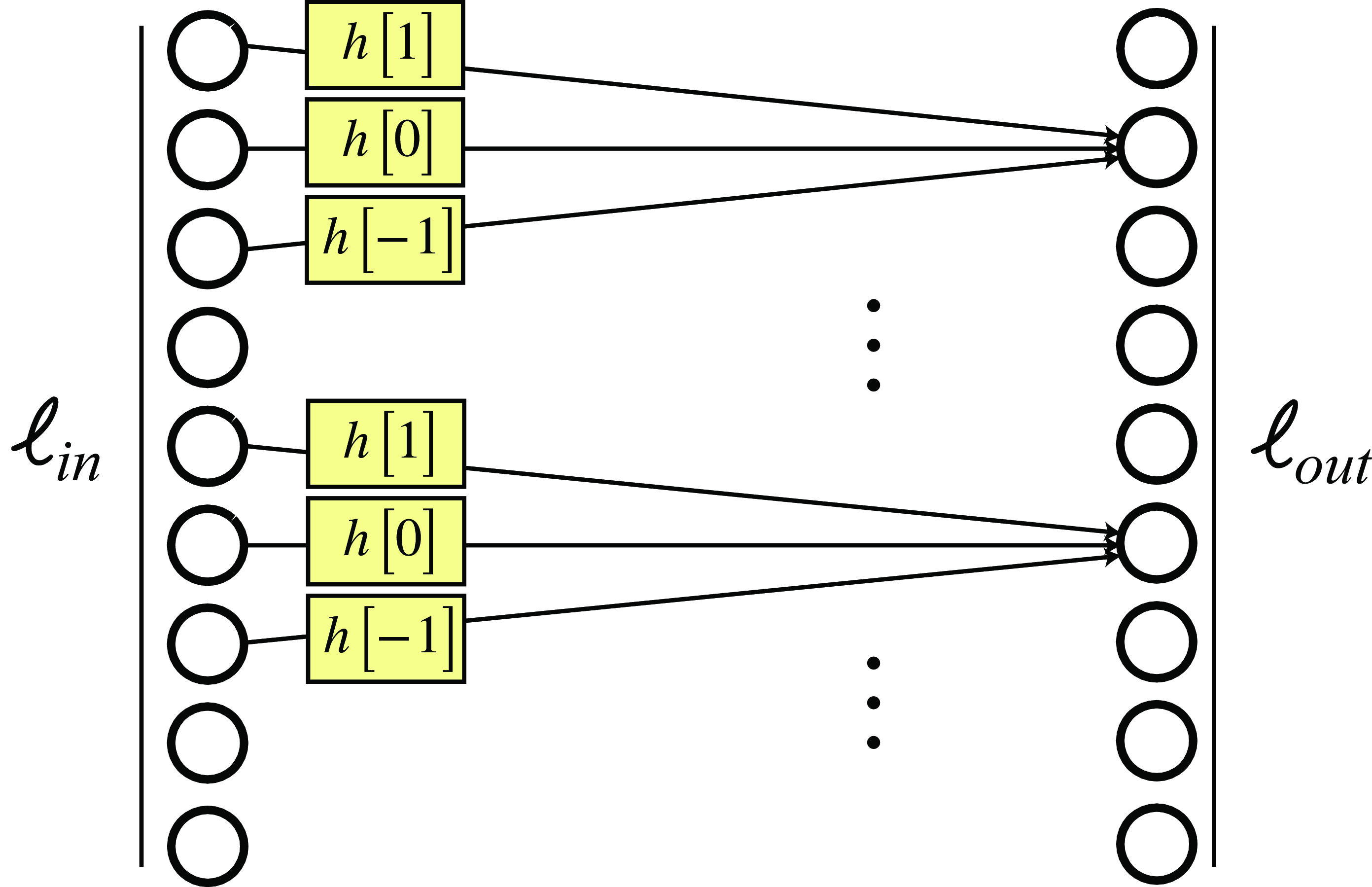
The convolution operation can be described in words as: first take the kernel \(h\left[k\right]\) and mirror it \(h\left[-k \right]\), then shift the mirrored kernel so that the origin is at location \(n\), then multiply the input values around location \(n\) by the mirrored kernel and sum the result. Store the result in the output vector \(\ell_{\texttt{out}}\left[n\right]\). For instance, if the convolutional kernel has three non-zero values: \(h\left[-1 \right] =1\), \(h\left[0 \right] = 2\) and \(h\left[1 \right] = 3\), then the output value at location \(n\) is \(\ell_{\texttt{out}}\left[n\right] = 3 \ell_{\texttt{in}}\left[n-1\right]+2 \ell_{\texttt{in}}\left[n\right] + 1 \ell_{\texttt{in}}\left[n+1\right]\). For finite length signals, it helps to make explicit the structure of the convolution writing it in matrix form. For instance, if the convolutional kernel has only three non-zero values, then: \[\begin{bmatrix} \ell_{\texttt{out}}\left[ 0 \right] \\ \ell_{\texttt{out}}\left[ 1 \right] \\ \ell_{\texttt{out}}\left[ 2 \right] \\ \vdots \\ \ell_{\texttt{out}}\left[ N-1 \right] \end{bmatrix} = \begin{bmatrix} h\left[0\right] ~&~ h\left[-1\right] ~&~ 0 ~&~ ... ~&~ 0 \\ h\left[1\right] ~&~ h\left[0\right] ~&~ h\left[-1\right] ~&~... ~&~ 0 \\ 0 ~&~ h\left[1\right] ~&~ h\left[0\right] ~&~... ~&~ 0 \\ \vdots ~&~ \vdots ~&~ \vdots ~&~ \vdots \\ 0 ~&~ 0 ~&~ 0 ~&~... ~&~ h\left[0\right] \end{bmatrix} ~ \begin{bmatrix} \ell_{\texttt{in}}\left[0\right] \\ \ell_{\texttt{in}}\left[1\right] \\ \ell_{\texttt{in}}\left[2\right] \\ \vdots \\ \ell_{\texttt{in}}\left[N-1\right] \end{bmatrix}\]
This operation is much easier to understand if we draw it as a convolutional layer of a neural network as shown in Figure 15.6:
In two dimensions, the processing is analogous: the input filter is flipped vertically and horizontally, then slid over the image to record the inner product with the image everywhere. Mathematically, this is: \[\ell_{\texttt{out}}\left[n,m\right] = h \left[n,m\right] \circ \ell_{\texttt{in}}\left[n,m\right] = \sum_{k,l}h \left[n-k,m-l \right] \ell_{\texttt{in}}\left[k,l \right] \tag{15.4}\]
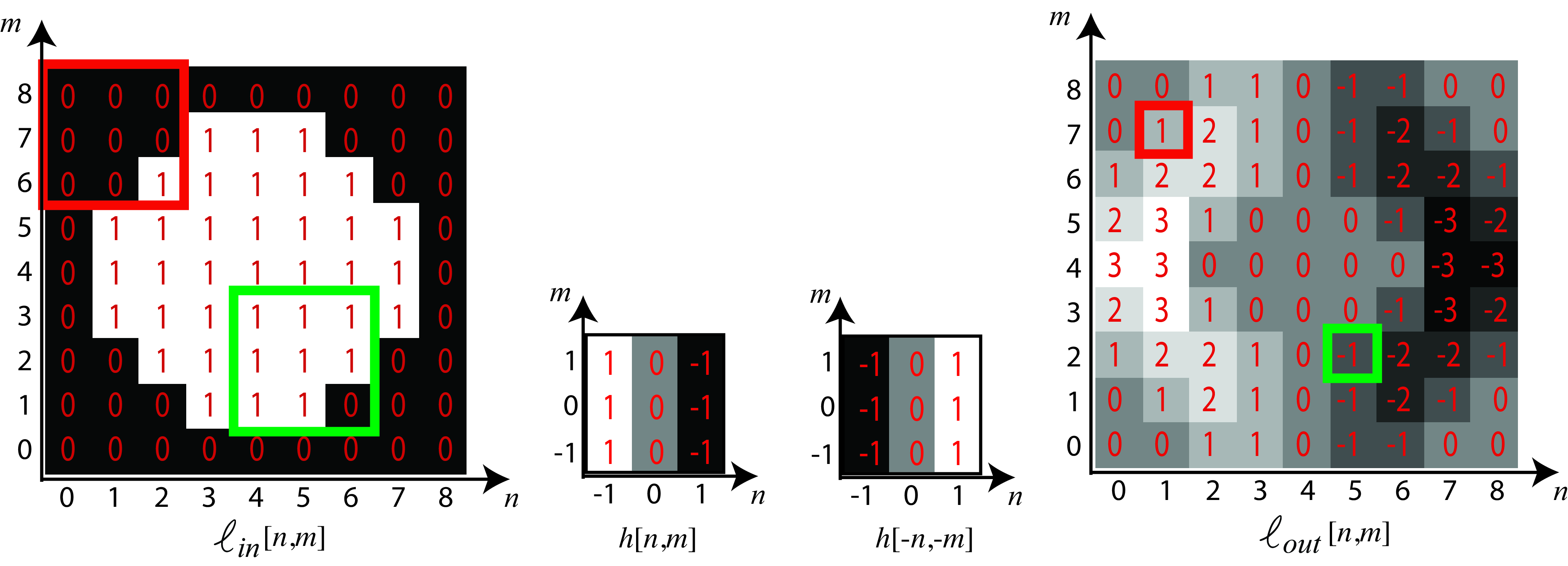
The next figure shows the result of a 2D convolution between a \(3 \times 3\) kernel with a \(9 \times 9\) image. The particular kernel used in the figure averages in the vertical direction and takes differences horizontally. The output image reflects that processing, with horizontal differences accentuated and vertical changes diminished. To compute one of the pixels in the output image, we start with an input image patch of \(3 \times 3\) pixels, we flip the convolutional kernel upside-down and left-right, and then we multiply all the pixels in the image patch with the corresponding flipped kernel values and we sum the results.
Let’s revisit the four image transformation examples from Figure 15.3 and ask a new question. Which ones of the image transformations shown in Figure 15.3 can be written as a convolution?
Only C and D from Figure 15.3 can be implemented by convolutions.
As shown in Figure 15.8 (a), in the defocusing transformation each output pixel at location \(n,m\) is the local average of the input pixels in a local neighborhood around location \(n,m\), and this operation is the same regardless of what pixel output we are computing. Therefore, it can be written as a convolution. The rotation transformation (for a fix rotation) is a linear operation but it is not translation invariant. As illustrated in Figure 15.8 (b), different output pixels require looking at input pixels in a way that is location specific. At the top left corner, one wants to grab a pixel from, say, five pixels up and to the right, and from the bottom right one needs to grab the pixel from about five pixels down and to the left. So this rotation operation can’t be written as a spatially invariant operation.
15.4.1 Properties of the Convolution
The convolution is a linear operation that will be extensively used thorough the book and it is important to be familiar with some of its properties.
Commutative. As we have already discussed before the convolution is commutative, \[h\left[n\right] \circ \ell\left[n\right] = \ell\left[n\right] \circ h\left[n\right]\] which means that the order of convolutions is irrelevant. This is not true for the correlation.
Associative. Convolutions can be applied in any order: \[\ell_1 \left[n\right] \circ \ell_2 \left[n\right] \circ \ell_3 \left[n\right] = \ell_1\left[n\right] \circ (\ell_2\left[n\right] \circ \ell_3\left[n\right]) = (\ell_1\left[n\right] \circ \ell_2\left[n\right]) \circ \ell_3\left[n\right] \tag{15.5}\] In practice, for finite length signals, the associative property might be affected by how boundary conditions are implemented.
Distributive with respect to the sum: \[\ell_1\left[n\right] \circ (\ell_2\left[n\right] + \ell_3\left[n\right] ) = \ell_1\left[n\right] \circ \ell_2\left[n\right] + \ell_1 \left[n\right] \circ \ell_3 \left[n\right]\]
Shift. Another interesting property involves shifting the two convolved functions. Let’s consider the convolution \(\ell_{\texttt{out}}\left[n\right] = h\left[n\right] \circ \ell_{\texttt{in}}\left[n\right]\). If the input signal, \(\ell_{\texttt{in}}\left[n\right]\), is translated by a constant \(n_0\), i.e. \(\ell_{\texttt{in}}\left[n - n_0\right]\), the result of the convolution with the same kernel, \(h\left[n\right]\), is the same output as before but translated by the same constant \(n_0\): \[\ell_{\texttt{out}}\left[n-n_0\right] = h\left[n\right] \circ \ell_{\texttt{in}}\left[n-n_0\right]\] Translating the kernel is equivalent: \[\ell_{\texttt{out}}\left[n-n_0\right] = h\left[n\right] \circ \ell_{\texttt{in}}\left[n-n_0\right] = h\left[n-n_0\right] \circ \ell_{\texttt{in}}\left[n\right]\]
Support. The convolution of a discrete signal of length \(N\) with another discrete signal of length \(M\) results in a discrete signal with length \(L \leq M+N-1\).
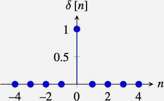
Identity. The convolution also has an identity function, that is the impulse, \(\delta \left[n\right]\), which takes the value 1 for \(n=0\) and it is zero everywhere else: \[\delta \left[n\right] = \begin{cases} 1 & \quad \text{if } n=0\\ 0 & \quad \text{if } n \neq 0 \\ \end{cases}\] The convolution of the impulse with any other signal, \(\ell\left[n\right]\), returns the same signal: \[\delta \left[n\right] \circ \ell\left[n\right] = \ell\left[n\right]\]
Given the signal:
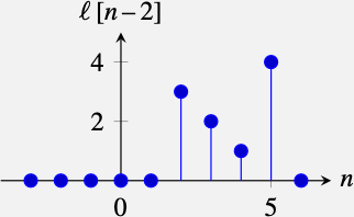
The signal \(\ell \left[n - n_0\right]\) is a shifted version of \(\ell \left[n\right]\). With \(n_0 = 2\) this is
The impulse function is
15.4.2 Some Examples
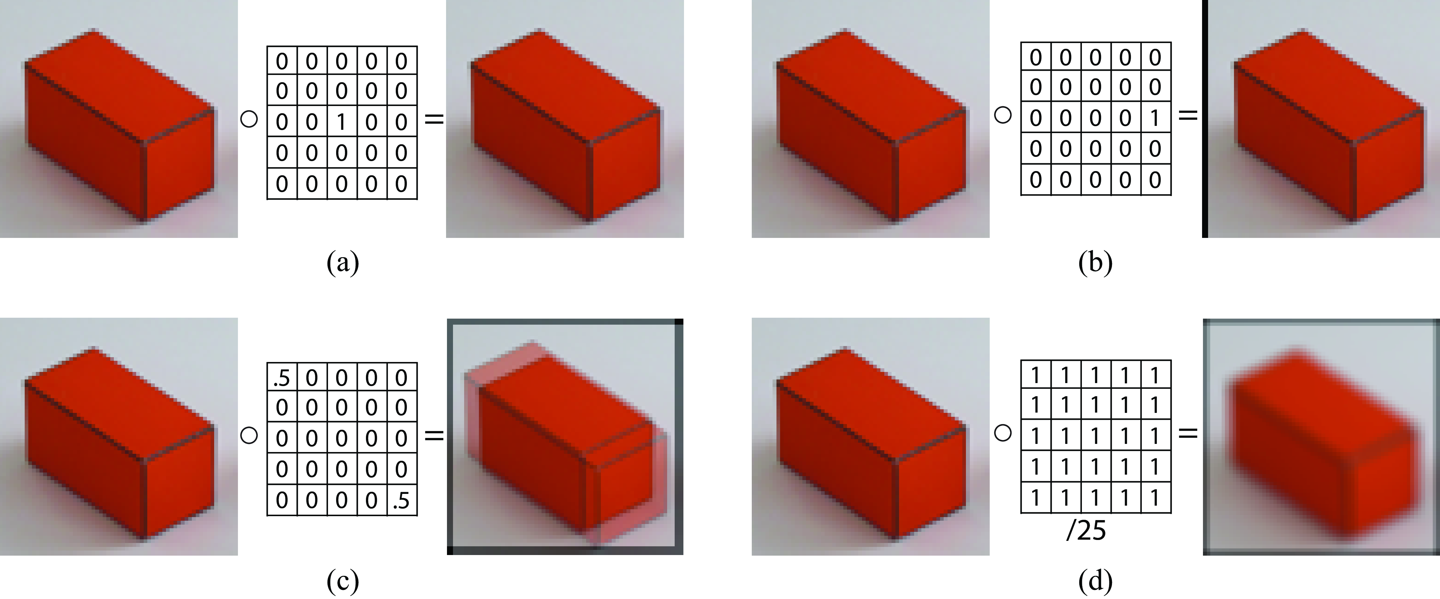
Figure 15.9 shows several simple convolution examples (each color channel is convolved with the same kernel). Figure 15.9 (a) shows a kernel with a single central non-zero element, \(\delta \left[n,m\right]\), convolved with any image, gives back that same image. Figure 15.9 (b) shows a kernel, \(\delta \left[n,m-2\right]\), that produces a two pixel shift toward the right of the input image. The black line that appears on the left is due to the zero-boundary conditions (to be discussed in the next section) and it has a width of two pixels. Figure 15.9 (c) shows the result of convolving the image with a kernel \(0.5 \delta \left[n-2,m-2\right]+ 0.5 \delta \left[n+2,m+2\right]\). This results in two superimposed copies of the same image shifted diagonally in opposite directions. And finally, Figure 15.9 (d) shows the result of convolving the image with a uniform kernel of all \(1/25\).
15.4.3 Handling Boundaries
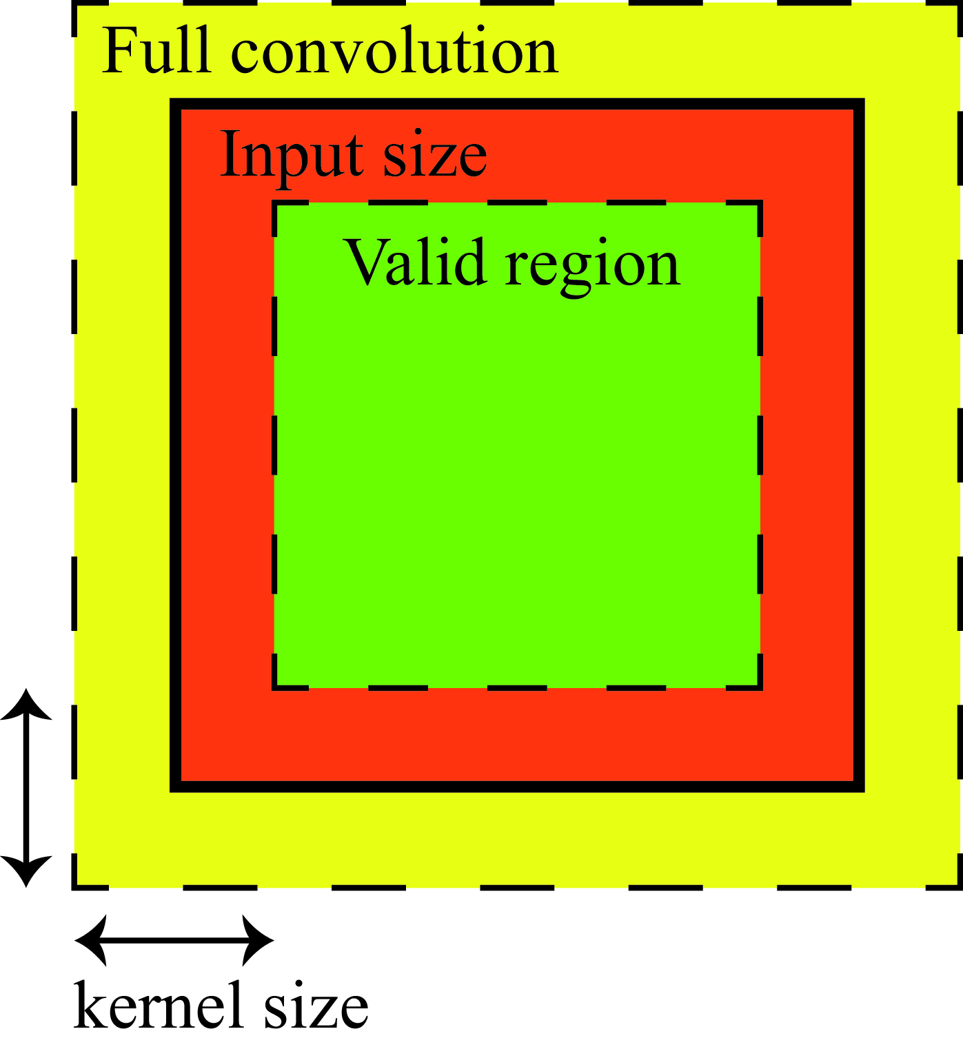
When implementing a convolution, one is confronted with the question of what to do at the image boundaries. There’s really no satisfactory answer for how to handle the boundaries that works well for all applications. One solution consists in omitting from the output any pixels that are affected by the input boundary. The issue with this is that the output will have a different size than the input and, for large convolutional kernels, there might be a large portion of the output image missing.
Only the green region contains values that can be computed, the rest will be affected by how we decide to handle the boundaries:
The most general approach consists in extending the input image by adding additional pixels so that the output can have the same size as the input. So, for a kernel with support \(\left[ -N, N \right] \times \left[-M, M\right]\), one has to add \(N\) additional pixels left and right of the image and \(M\) pixels at the top and bottom. Then, the output will have the same size as the original input image.
Some typical choices for how to pad the input image are (see Figure 15.10):
Zero padding: Set the pixels outside the boundary to zero (or to some other constant such as the mean image value). This is the default option in most neural networks.
Circular padding: Extend the image by replicating the pixels from the other side. If the image has size \(P \times Q\), circular padding consists of the following: \[\ell_{\texttt{in}}\left[n,m\right] = \ell_{\texttt{in}}\left[(n)_P,(m)_Q\right]\] where \((n)_P\) denotes the modulo operation and \((n)_P\) is the reminder of \(n/P\).
This padding transform the finite length signal into a periodic infinite length signal. Although this will introduce many artifacts, it is a convenient extension for analytical derivations.
Mirror padding: Reflect the valid image pixels over the boundary of valid output pixels. This is the most common approach and the one that gives the best results.
Repeat padding: Set the value to that of the nearest output image pixel with valid mask inputs.
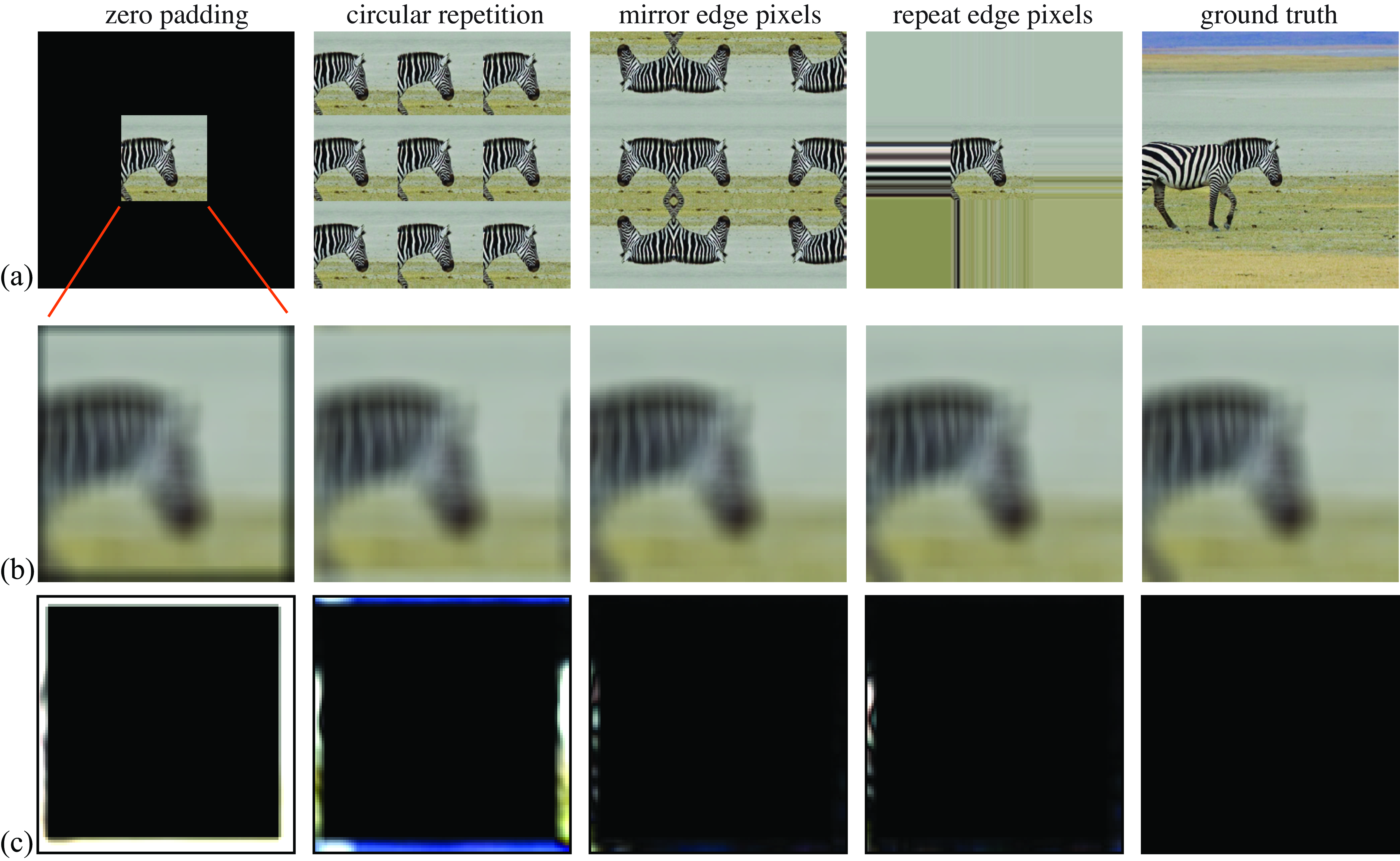
Figure 15.10 shows different examples of boundary extensions. Boundary extensions are different ways of approximating the ground truth image that exists beyond the image boundary. The top row shows how the image is extended beyond its boundary when using different types of boundary extensions (only the central part corresponds to the input). The middle row shows the output of the convolution (cropped to match the size of the input image). We can see that the zero-padding makes a darkening appear on the boundary of the image. This is not very desirable in general. The other padding methods seem to produce better visual results.
But which one is the best boundary extension? Ideally, we would to get a result that is a close as possible to the output we would get if we had access to a larger image. In this case we know what the larger image looks like as shown in the last column of Figure 15.10. For each boundary extension method, the final row shows the absolute value of the difference between the convolution output and the result obtained with the ground truth.
For the example of Figure 15.10, the error seems to be smaller when extending the image using mirror padding. On the other extreme, zero padding seems to be the worst.
15.4.4 Circular Convolution
Writing the circular convolution in matrix form will look like: 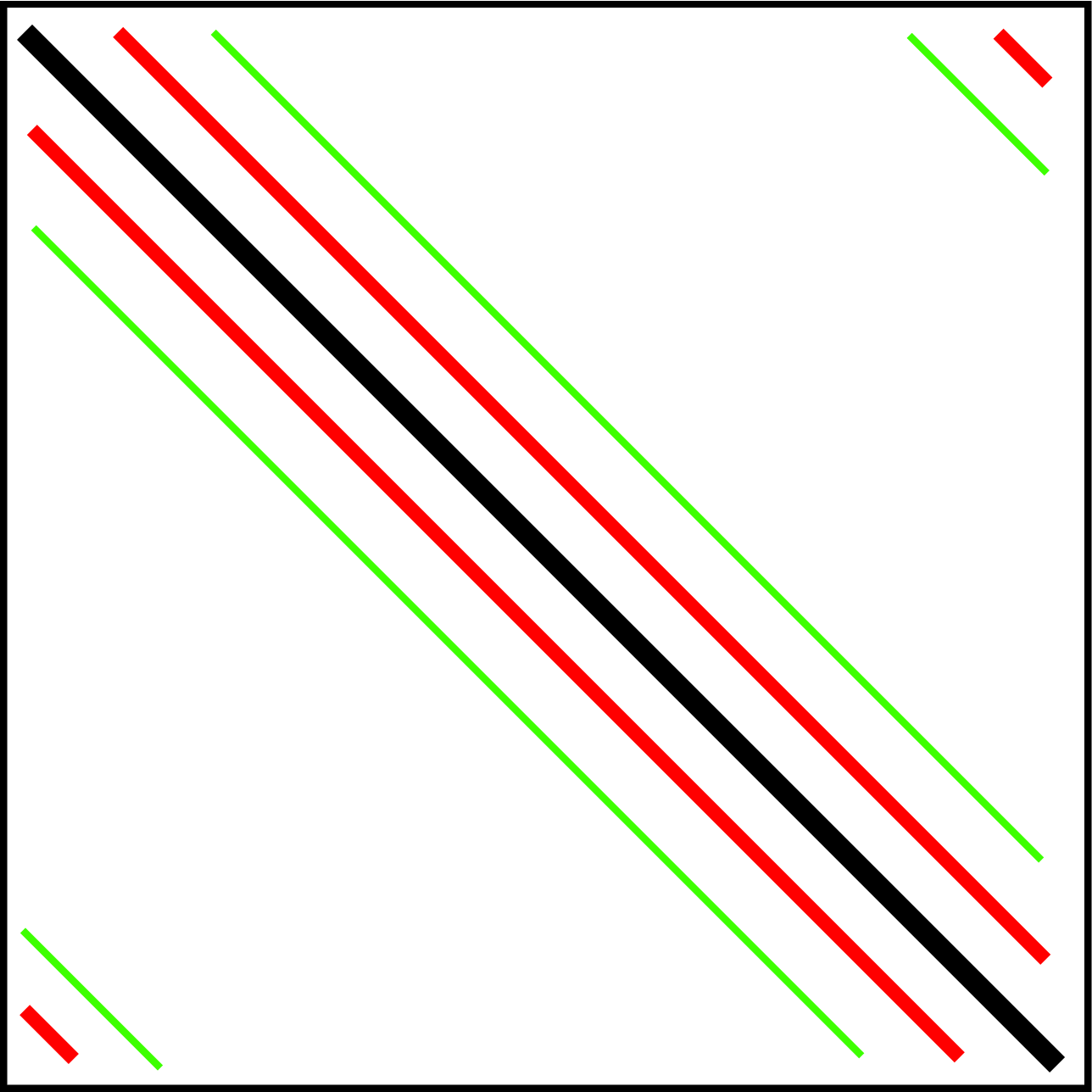
When convolving a finite length signal with a kernel, we have seen that it can be convenient to extend the signal beyond its boundary to reduce boundary artifacts. This trick is also very useful analytically and conduces to a special case of the convolution: the circular convolution uses circular padding. The circular convolution of two signals, \(h\) and \(\ell_{\texttt{in}}\), of length \(N\) is defined as follows:
\[\ell_{\texttt{out}}\left[n\right] = h \left[n\right] \circ_N \ell_{\texttt{in}}\left[n\right] = \sum_{k=0}^{N-1} h \left[(n-k)_N \right] \ell_{\texttt{in}}\left[k \right]\]
In this formulation, the signal \(h \left[ (n)_N \right]\) is the infinite periodic extension, with period \(N\), of the finite length signal \(h \left[n \right]\). The output of the circular convolution is a periodic signal with period \(N\), \(\ell_{\texttt{out}}\left[n \right] = \ell_{\texttt{out}}\left[(n)_N \right]\).
The circular convolution has the same properties than the convolution (e.g., is commutative.)
15.4.5 Convolution in the Continuous Domain
The convolution in the continuous domain is defined in the same way as with discrete signals but replacing the sums by integrals. Given two continuous signals \(h(t)\) and \(\ell_{\texttt{in}}(t)\), the convolution operator is defined as follows: \[\ell_{\texttt{out}}(t) = h(t) \circ \ell_{\texttt{in}}(t) = \int_{-\infty}^{\infty} h(t-\tau) \ell_{\texttt{in}}(\tau) d\tau\]
The properties of the continuous domain convolution are analogous to the properties of the discrete convolution, with the commutative, associative and distributive relationships still holding.
We can also define the impulse, \(\delta (t)\), in the continuous domain such that \(\ell(t) \circ \delta(t) = \ell(t)\).
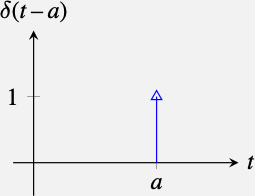
The impulse is defined as being zero everywhere but at the origin where it takes an infinitely high value so that its integral is equal to 1: \[\int_{-\infty}^{\infty} \delta(t) dt = 1\] The impulse function is also called the impulse distribution (as it is not a function in the strict sense) or the Dirac delta function.
The delta distribution is usually represented with an arrow of height 1, indicating that it has an finite value at that point, and a finite area equal to 1:
The impulse has several important properties:
Scaling property: \(\delta (at) = \delta (t) / |a|\)
Symmetry: \(\delta (-t) = \delta (t)\)
Sampling property: \(\ell(t) \delta (t-a) = \ell(a) \delta (t-a)\) where \(a\) is a constant. From this, we have the following: \[\int_{-\infty}^{\infty} \ell(t) \delta (t-a) dt = \ell(a)\]
As in the discrete case, the continuous impulse is also the identity for the convolution: \(\ell(t) \circ \delta (t) = \ell(t)\).
The impulse will be useful in analytical derivations and we will see it again in chapter Chapter 20 when we discuss sampling.
15.5 Cross-Correlation Versus Convolution
Another form of writing a translation invariant filter is using the cross-correlation operator. The cross-correlation provides a simple technique to locate a template in an image. The cross-correlation and the convolution are closely related.
The cross-correlation operator (denoted by \(\star\)) between the image \(\ell_{\texttt{in}}\) and the kernel \(h\) is written as follows: \[\ell_{\texttt{out}}\left[n,m\right] = \ell_{\texttt{in}}\star h = \sum_{k,l=-N}^N \ell_{\texttt{in}}\left[n+k,m+l \right] h \left[k,l \right]\] where the sum is done over the support of the filter \(h\), which we assume is a square \((-N,N)\times(-N,N)\). In the convolution, the kernel is inverted left-right and up-down, while in the cross-correlation is not. Remember that the convolution between image \(\ell_{\texttt{in}}\) and kernel \(h\) is written as follows: \[\ell_{\texttt{out}}\left[n,m\right] = \ell_{\texttt{in}}\circ h = \sum_{k,l=-N}^N \ell_{\texttt{in}}\left[n-k,m-l \right] h \left[k,l \right]\]
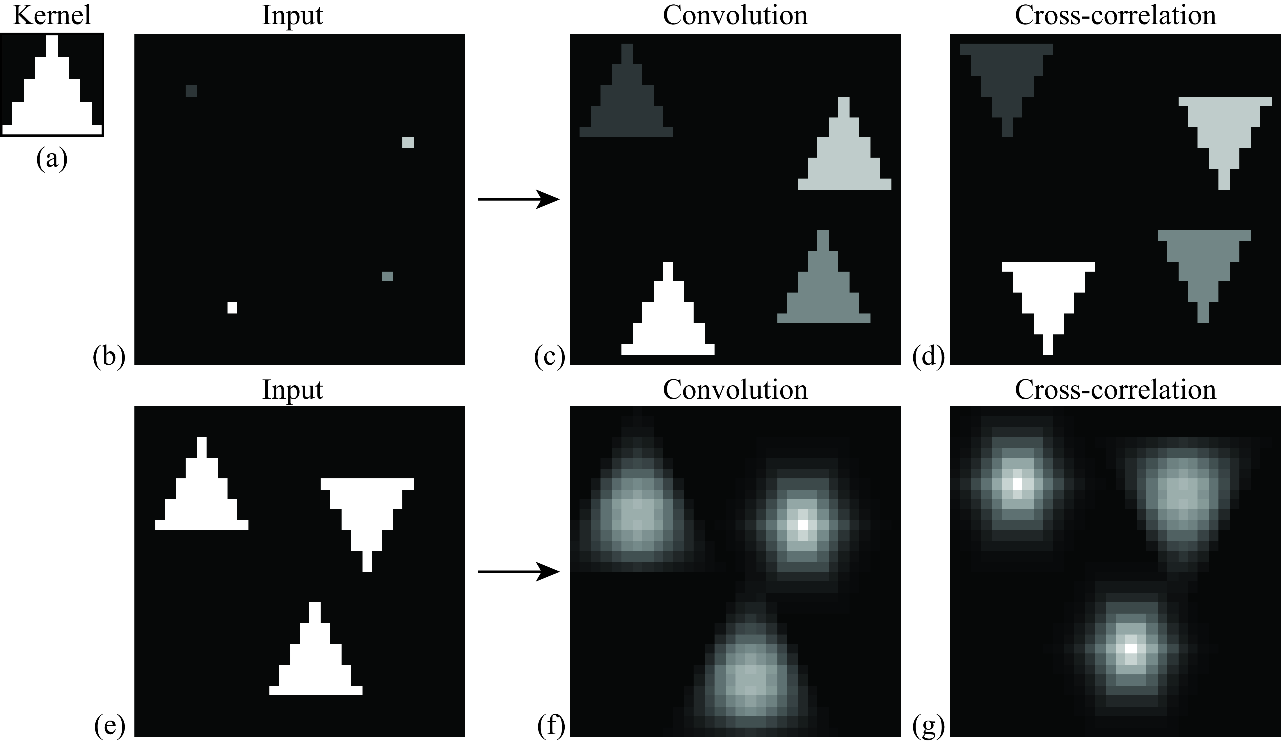
Figure 15.11 illustrates the difference between the correlation and the convolution. In these examples, the kernel \(h[n,m]\) is a triangle pointing up (the center of the triangle is \(n=0\) and \(m=0\)) as shown in Figure 15.11 (a). When the input image is black (all zeros) with only four bright pixels, Figure 15.11 (b), this is the convolution of the triangle with four impulses, which results in four triangles pointing up (Figure 15.11[c]). However, the cross-correlation looks different; it still results in four copies of the triangles centered on each point, but the triangles are pointing downward (Figure 15.11[d]).
For the input image containing triangles pointing up and down, Figure 15.11 (e), the convolution will have its maximum output on the triangles points down, Figure 15.11 (f), while the correlation will output the maximum values in the center of the triangles pointing up (Figure 15.11[g]).
Another important difference between the two operators is that the convolution is commutative and associative while the correlation is not. The correlation breaks the symmetry between the two functions \(h\) and \(\ell_{\texttt{in}}\). For instance, in the correlation, shifting \(h\) is not equivalent to shifting \(\ell_{\texttt{in}}\) (the output will move in opposite directions). Note that the cross-correlation and convolution outputs are identical when the kernel \(h\) has central symmetry.
15.5.1 Template Matching and Normalized Correlation
The goal of template matching is to find a small image patch within a larger image. Figure 15.12 shows how to use template matching to detect all the occurrences of the letter “a” with an image of text, shown in Figure 15.12 (b). Figure 15.12 (a) shows the template of the letter “a”.
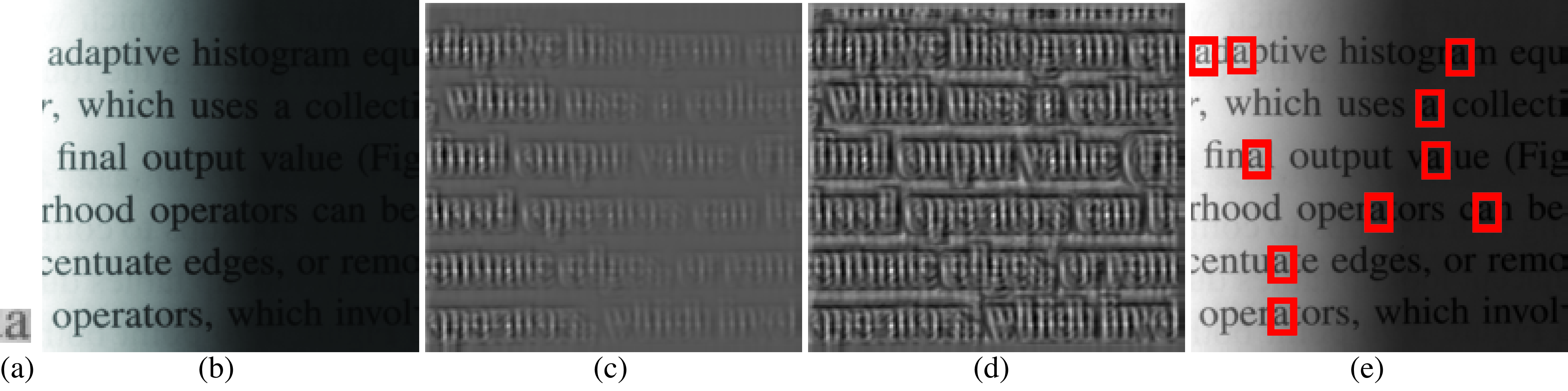
Cross-correlation is a potential method for template matching, but it has certain flaws. Consider matching the “a” template in Figure 15.12 (a) in a given input image. Just by increasing the brightness of the image in different parts we can increase the filter response since correlation is essentially a multiplication between the kernel \(h\) and any input image patch \(p\) (note that all the values are positive in \(p\) and \(h\)). In bright image regions we will have the maximum correlation values regardless of regions’ content as shown in Figure 15.12 (c).
The normalized cross-correlation, at location \((n,m)\), is the dot product between a template, \(h\), (normalized to be zero mean and unit norm) and the local image patch, \(p\), centered at that location and with the same size as the kernel, normalized to be unit norm. This can be implemented with the following steps: First, we normalize the kernel \(h\). The normalized kernel \(\hat h\) is the result of making the kernel \(h\) zero mean and unit norm. Then, the normalized cross-correlation is as follows (Figure 15.12 (d)):
\[\ell_{\texttt{out}}\left[n,m\right] = \frac{1}{\sigma \left[n,m \right]} \sum_{k,l=-N}^N \ell_{\texttt{in}}\left[n+k,m+l \right] \hat{h} \left[k,l \right]\]
Note that this equation is similar to the correlation function, but the output is scaled by the local standard deviation, \(\sigma \left[m,n \right]\), of the image patch centered in \((n,m)\) and with support \((-N,N)\times(-N,N)\), where \((-N,N)\times(-N,N)\) is the size of the kernel \(h\). To compute the local standard deviation, we first compute the local mean, \(\mu \left[n,m \right]\), as follows: \[\mu \left[n,m \right] = \frac{1}{(2N+1)^2} \sum_{k,l=-N}^N \ell_{\texttt{in}}\left[n+k,m+l \right]\] And then we compute: \[\sigma^2 \left[n,m \right] = \frac{1}{(2N+1)^2} \sum_{k,l=-N}^N \left( \ell_{\texttt{in}}\left[n+k,m+l \right] - \mu \left[n,m \right] \right) ^2\]
Figure 15.12 (e) shows the detected copies of the template Figure 15.12 (a) in the image Figure 15.12 (b). The red bounding boxes in Figure 15.12 (e) correspond to the location with local maximum values of the normalized cross-correlation (Figure 15.12 (d) that are above a threshold chosen by hand.
In the example of Figure 15.12, all the instances of the letter ‘a’ have been correctly detected. But this method is very fragile when used to detect objects and is useful only under very limited conditions. Normalized correlation will detect the object independently of location, but it will not be robust to any other changes such as rotation, scaling, and changes in appearance. Just changing the font of the letters will certainly make the approach fail.
15.6 System Identification
One important task that we will study is that of explaining the behavior of complex systems such as neural networks. For an LTI filter with kernel \(h\left[n\right]\), the output from an impulse is \(y\left[n\right] = h\left[n\right]\). The output of a translated impulse \(\delta \left[n -n_0 \right]\) is \(h \left[n -n_0 \right]\). This is why the kernel that defines an LTI system, \(h\left[n\right]\), is also called the impulse response of the system.
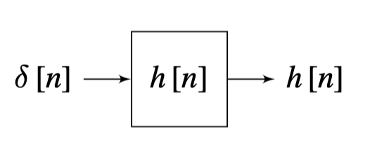
For an unknown system, one way of finding the convolution kernel \(h\) consists in computing the output of the system when the input is an impulse.
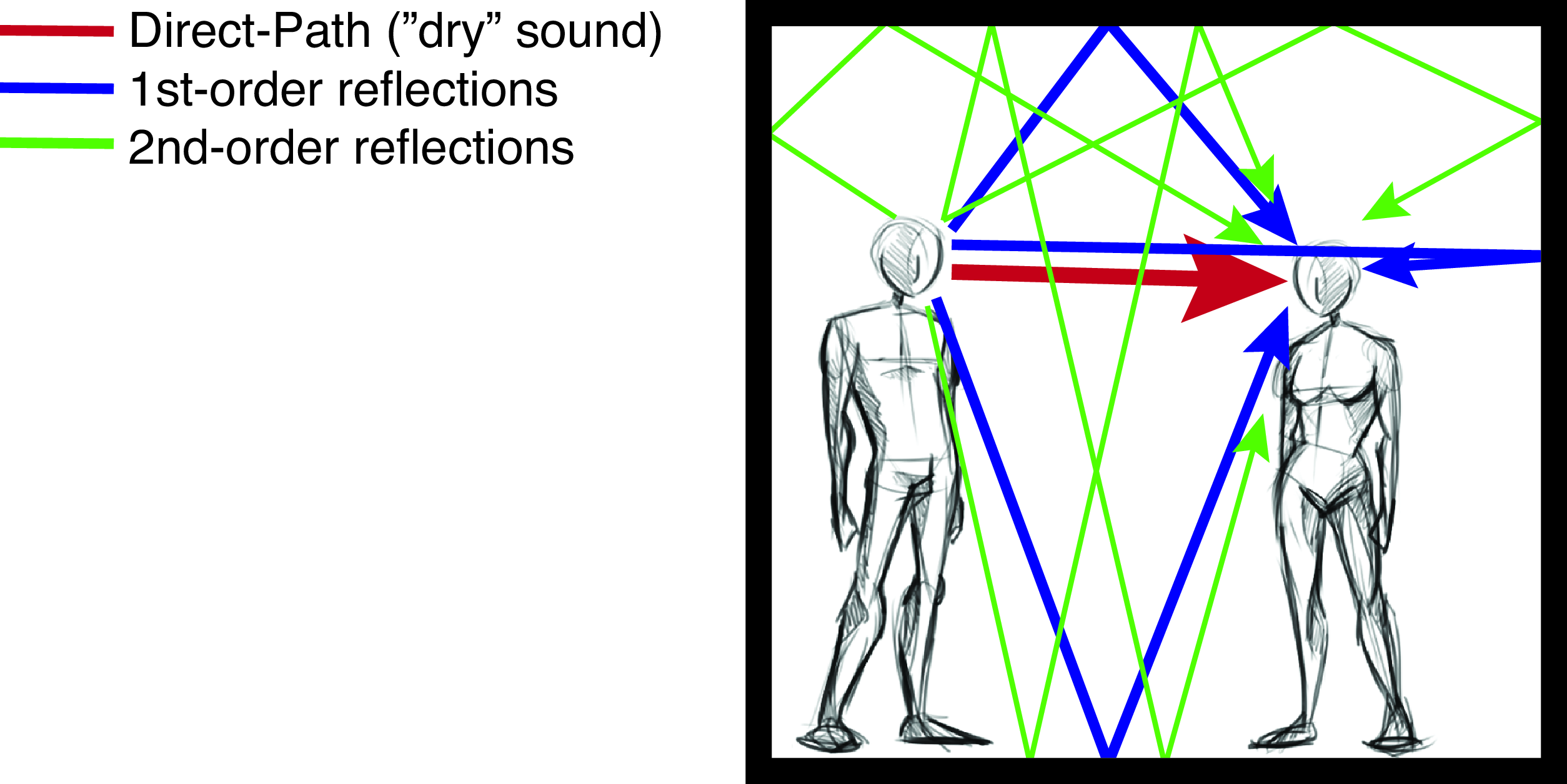
Let’s start with a beautiful example from acoustics [3]. When you are in a room you often hear that sounds are distorted with echos (Figure 15.14). The number and strength of the echos depend on the geometry of the room, whether it is full or empty and the materials in the walls and ceilings.
Interestingly the relationship between the sounds that are originated in one location and what a listener hears in another position are related by an LTI system. If you are in a room and you clap (which is a good approximation to an impulse of sound), the echoes that you hear are very close to the impulse response of the system formed by the acoustics of the room. Any sounds that originates at the location of your clap will produce a sound in the room that will be qualitatively similar to the convolution of the acoustic signal with the echoes that you hear before when you clapped. Figure 15.15 shows a recording made in a restaurant in Cambridge, Massachusetts.
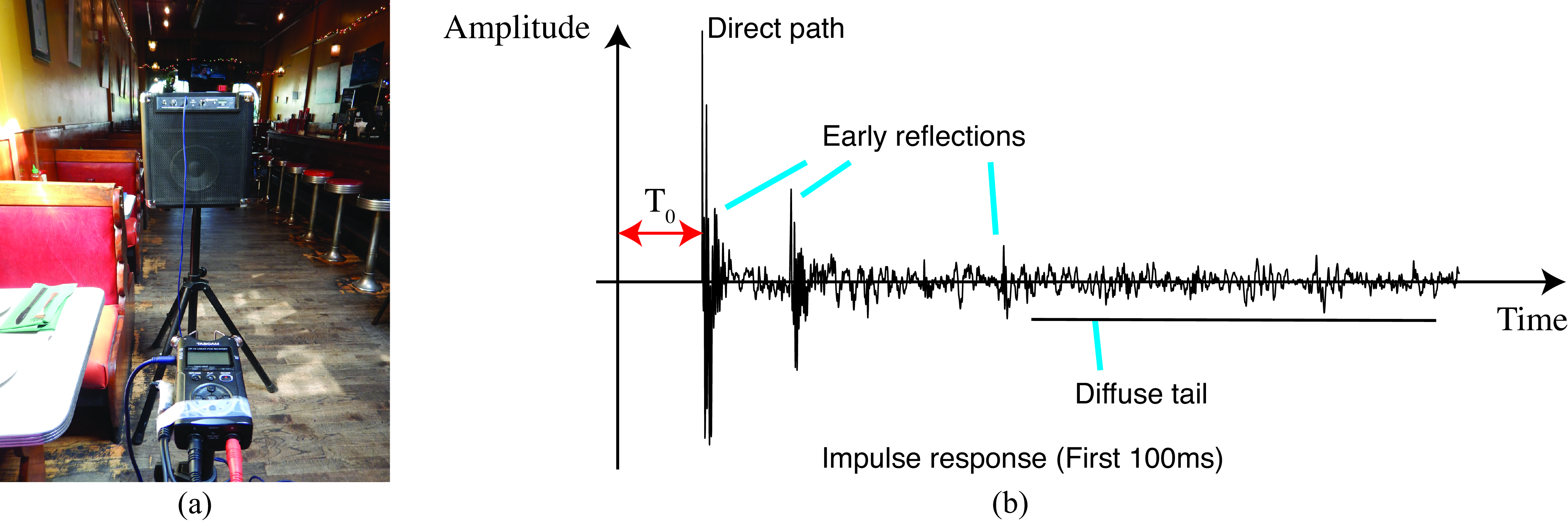
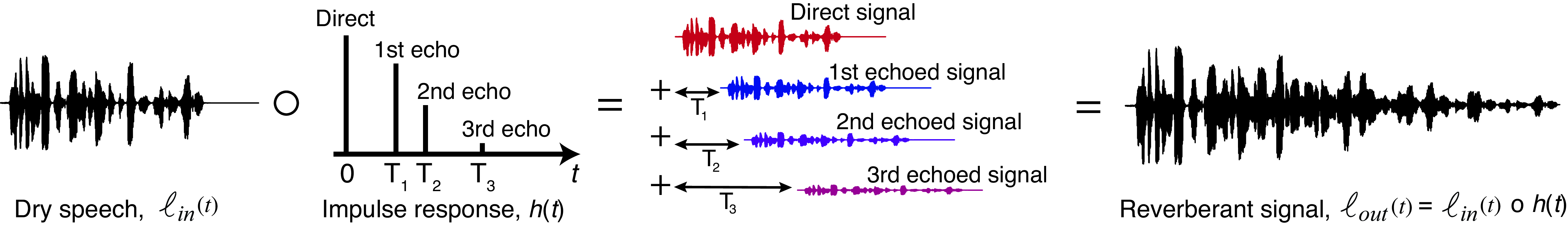
Figure 15.16, adapted from [3], shows a sketch of how a voice signal gets distorted by the impulse response of a room before it reaches the listener. The impulse response, \(h (t)\), is modeled here as a sequence of four impulses, the first impulse corresponds to the direct path and the remaining three to the different paths inside the room, modeled with different delays (\(T_i\)) and amplitudes (\(0 < a_i < 1\)):
\[h (t) = a_0 \delta (t) + a_1 \delta \left(t-T_1 \right) + a_2 \delta \left( t-T_2 \right) + a_3 \delta \left( t-T_3 \right)\]
The sound that reaches the listener is the superposition of four copies of the sound emitted by the speaker. This can be written as the convolution of the input sound, \(\ell_{\texttt{in}}(t)\), with room impulse response, \(h (t)\): \[\ell_{\texttt{out}}(t) = \ell_{\texttt{in}}(t) \circ h(t) = a_0 \ell_{\texttt{out}}(t) + a_1 \ell_{\texttt{in}}(t-T_1) + a_2 \ell_{\texttt{in}}(t-T_2) + a_3 \ell_{\texttt{in}}(t-T_3)\] which is shown graphically in Figure 15.16.
15.7 Concluding Remarks
A good foundation in signal processing is a valuable background for computer vision scientists and engineers. This short introduction should now allow you go deeper by consulting other specialized books.
But we are not done yet. In the next chapter we will study the Fourier transform, which will provide a useful characterization of signals and images.