46 Motion Estimation
46.1 Introduction
An important task in both human and computer vision is to model how images (and the underlying scene) change over time. Our visual input is constantly moving, even when the world is static. Motion tells us how objects move in the world, and how we move relative to the scene. It is an important grouping cue that lets us discover new objects. It also tells us about the three-dimensional (3D) structure of the scene.
Look around you and write down how many things are moving and what are they doing. Take note of the things that are moving because you interact with them (such as this book or your computer) and the things that move independently of you.
The first observation you might make is that not much is happening. Nothing really moves. Most of the world is remarkably static, and when something moves it attracts our attention. However, motion perception becomes extremely powerful as soon as the world starts to move. Our visual system can form a detailed representation of moving objects with complex shapes. Even in front of a static image, we form a representation of the dynamics of an object, as shown in the photograph in Figure 46.1.

Looking at the power of that static image to convey motion, one wonders if seeing movies is really necessary. From the notes you took about what moves around you, probably you deduced that the world is, most of the time, static.
And yet, biological systems need motion signals to learn. Hubel and Wiesel [1] observed that a paralyzed kitten was not capable of developing its visual system properly. The human eye is constantly moving with saccades and microsaccades. Even when the world is static, the eye is a moving camera that explores the world. Motion tells us about the temporal evolution of a 3D scene, and is important for predicting events, perceiving physics, and recognizing actions. Motion allows us to segment objects from the static background, understand events, and predict what will happen next. Motion is also an important grouping cue that our visual system uses to understand what parts of the image are connected. Similarly moving scene points are likely to belong to the same object. For example, the movement of a shadow accompanying an object, or various parts of a scene moving in unison—even when the connecting mechanism is concealed—strongly suggests that they are physically linked and form a single entity.
Motion estimation between two frames in a sequence is closely related to disparity estimation in stereo images. A key difference is that stereo images incorporate additional constraints, as only the camera moves—imagine a stereo pair as a sequence with a moving camera while everything else remains static. The displacements between stereo images respect the epipolar constraint, which allows the estimated motions to be more robust. In contrast, optical flow estimation doesn’t assume a static world.
Disparity from stereo and optical flow estimations are closely related. Stereo benefits from the epipolar constraint to make estimation easier. For a rectified stereo pair the vertical component of motion between the stereo frames is zero.
Another distinction is that optical flow generally presumes small displacements between consecutive frames due to the short time gap between them. In stereo images, feature displacements tend to be larger. Despite these differences, the remaining steps are similar, and the same architectures can address both tasks.
46.2 Motion Perception in the Human Visual System
The eye is constantly moving, fixating different scene locations every 300 ms. Therefore, the nature of the input signal to the brain is a sequence of ever-changing visual information. It is not a surprise then that motion perception is a key component of visual perception.
Only when the eye tracks a moving object can it move continuously. Otherwise, the eye jumps from one location to another in saccades. Try moving your eyes smoothly and you will notice that you cannot. However, if you look at your finger you will see that you can follow its motion smoothly.
What do we know about the human perception of motion? Much is known and many advances from cognitive psychology have impacted imaging technology. One example is movies. The fact that we learned to create the illusion of continuous motion by displaying a sequence of static images (a phenomenon called apparent motion) was a remarkable discovery.
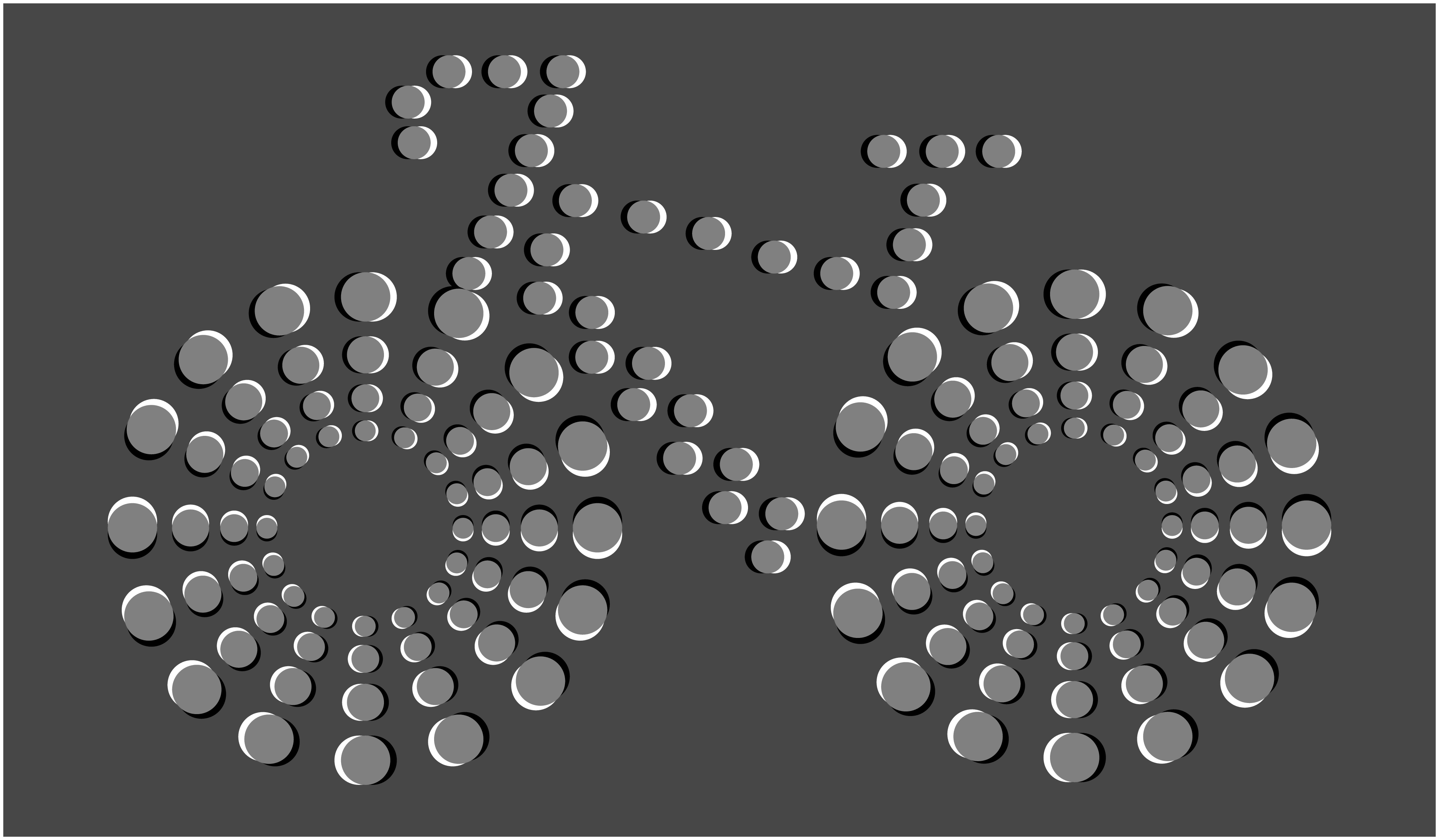
There are a number of visual illusions associated with motion perception that are intriguing and offer a window into how motion perception is implemented in the brain. One famous illusion is the waterfall illusion. When looking at a constant motion (such as a waterfall) our brain adapts to the motion in such a way that if, immediately after adaptation, we look at a static texture we will see it drifting in the opposite direction. The waterfall illusion was already known to the Greeks and was reported by Aristotle. Another remarkable and surprising visual illusion is that it is possible to create static images that produce the sensation of motion. One beautiful example is the Rotating Snakes visual illusion created by cognitive psychologist Akiyoshi Kitaoka. Figure 46.2 shows an example a motion-inducing visual illusion, using very simple elements to produce the illusion. The effect becomes more intense as we move our eyes to explore different parts of the bicycle.
The opposite visual illusion can also be achieved: perceiving no motion when there is movement. By creating sequences with isoluminant and textureless patterns [3], an observer can perceive them as perfectly still, even though they are moving. This illusion requires precise calibration and only works for the specific observer the system is tuned for; other observers will still see motion. The illusion can be thought of as an adversarial attack on a single observer’s motion estimation system. What mechanisms does the brain use to translate the sequence of images projected on the retina into actual motion in the 3D scene? This question has long been studied by neuroscientists and psychologists.
In area V1 of the visual cortex, most visual neurons respond to moving stimuli and exhibit selectivity to specific motion directions. A motion-selective neuron responds strongly when an edge moves across its receptive field in a particular orientation, and its response diminishes as the motion deviates from the preferred direction. These motion-selective cells project to other specialized areas, with the middle temporal area (area MT) and the medial superior temporal area (area MST) playing significant roles in motion processing. The exact functions and roles of these areas are not yet fully understood. This organization suggests that motion is processed by specialized visual pathways, indicating a modular architecture for the visual system.
One of the early computational models of motion perception was proposed by Hassenstein and Reichardt [4] when studying the motion detectors in the fly’s visual system. Another computational model of human motion perception is the energy model proposed by Adelson and Bergen [5] and briefly discussed in Chapter 22. In this chapter we will focus on motion estimation algorithms developed by the computer vision community without trying to follow biologically plausible mechanisms.
46.3 Matching-Based Motion Estimation
Let’s get our hands dirty quickly by trying to estimate how pixels move in a video. Let’s consider two frames of a video sequence that contains a few moving objects, as shown in Figure 46.3.
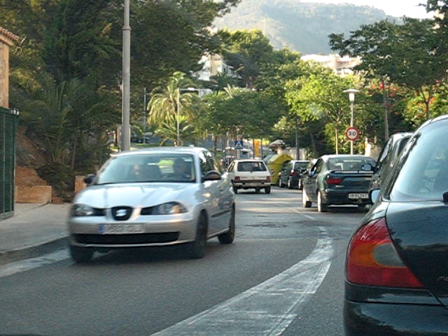
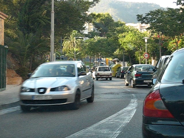
These two frames belong to a sequence captured from a moving car driving along a busy street. In this sequence there are cars moving on both sides of the road, some moving away from the camera and others moving toward it. How can we compute the motion between the two frames? One way of representing the motion is by computing the displacement for each pixel between the two frames.
Under this formulation, the task of motion estimation consists of finding, for each pixel in frame 1, the location of the corresponding pixel in frame 2. Just as in the chapter on stereo matching, we need first to define how we will compare pixels to find correspondences.
Using the color of each individual pixel will be insufficient as many pixels are likely to have very similar colors. Instead we will represent each pixel by a color patch of size \(C=3\times(2s+1)\times(2s+1)\) centered on each pixel. That is, for pixel in location \((n,m)\) in image \(\boldsymbol\ell\), we will use the patch \(\boldsymbol\ell[n-s:n+s, m-s:m+s]\) to represent the local appearance in that location. Small values of \(s\) will result is small patches that might be less distinctive (\(s=0\) corresponds to use individual pixels), while large values of \(s\) will result in large discriminative patches but might fail if there is sufficient geometric distortion between the two frames due to motion. By representing each pixel with a patch, we are transforming the image into a feature map of size \(3\times(2s+1)\times(2s+1)\). As in Chapter 31, we could also use other patch embeddings such as DINO or SIFT descriptors. But since the image transformation between two consecutive frames is usually small, using red-green-blue (RGB) patches can work well. Another constraint we can use to simplify the matching is to assume that motion will be small between the two frames so that we only need to look for matches inside a small neighborhood of size \(L \times L\) in the second frame around the original pixel location. To compute distances between two patches we will use the Euclidian distance between them. We will then compute the motion at each pixel in the first frame by searching for the patch with the smallest distance in the second frame. We can implement this with the following algorithm:
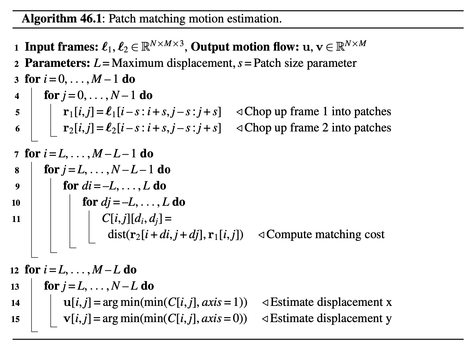
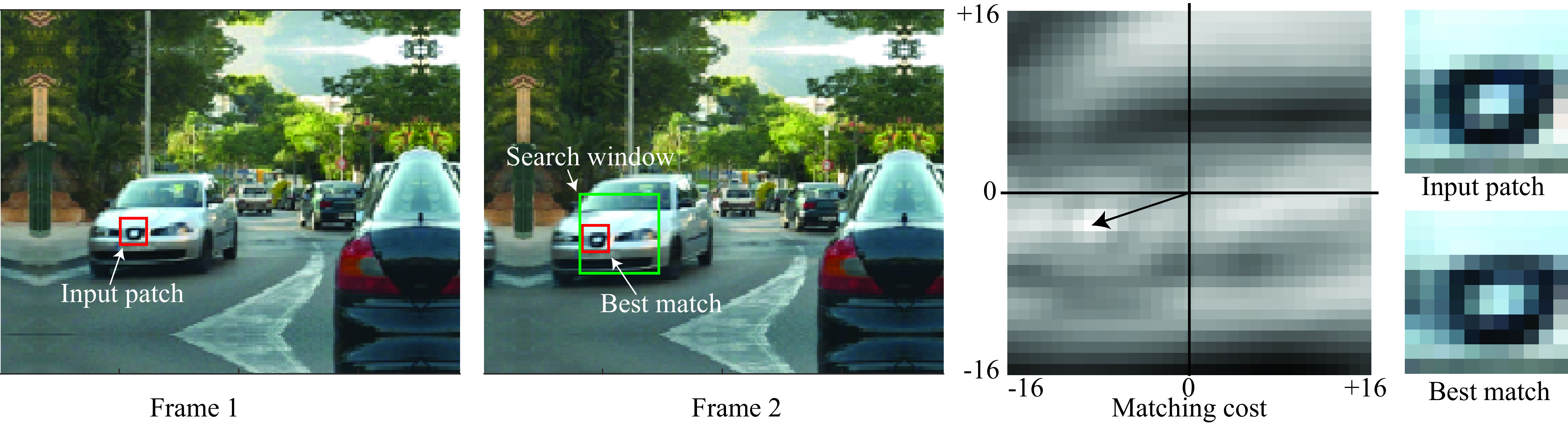
Note that padding must be applied if we want to compute the output optical flow near the image boundaries. Algorithm Algorithm 46.1 could be written more compactly but we prefer this form for its clarity. The following images shows the matching result for one input location. In this example, \(s=5\) (patch size of \(11\times11\) pixels), and \(L=16\) (search window of size \(33\times33\) pixels).
In the example shown in Figure 46.4, the input patch is centered on the car logo. The matching cost displays the distance using a reversed grayscale map, with smaller values appearing as brighter spots. In this case, the search identifies a unique match. However, it is worth noting that the best matching patch, although correctly detecting the same logo, is not identical to the input patch. This discrepancy can be attributed to factors such as nondiscrete motion and the slight enlargement of the logo as the car approaches the camera.
The patch size used to represent each pixel is the most important parameter in this algorithm. Figure 46.5 shows the effect of the choice of the parameter \(s\) on the estimated optical flow.
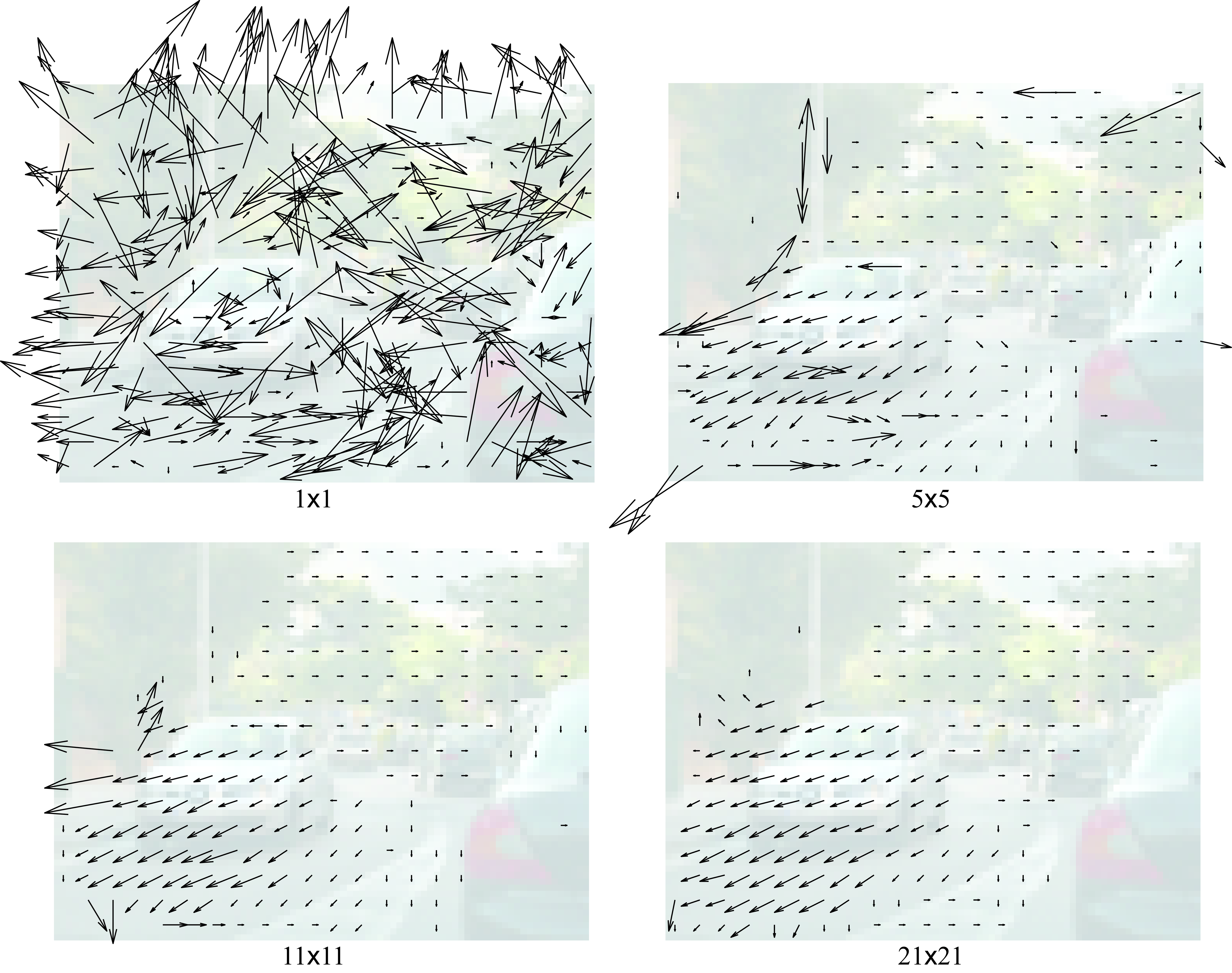
When using single pixels to represent each location, the matching fails in detecting true correspondences and the estimated motion field is very noisy. Just making the patches \(5 \times 5\) pixels is already capable of detecting many correct matches and the motion field seems to mostly capture the true motion between the two frames. Further increasing the patch size eliminates some of the errors. However, using very big patches also introduces new problems. In this example we can see how the motion of the gray car extends over the road. This is due to patches overlapping with the car on top, and as the road is mostly uniform, the motion of the car propagates to all the nearby pixels. One of the challenges in this algorithm is that the ideal value of \(s\) will depend on the sequence.
This approach has many shortcomings. To start, we assumed that motion is discrete (it can only take on integer values). Therefore, the current approach does not compute displacements of pixels to subpixel accuracy that might be important if we need precision or if motions are very small. We could improve the approach by interpolating the cost function or by computing subpixel displacements using bilinear or bicubic interpolation, but it would become more computationally expensive. In addition, the patch matching method gives poor results near motion discontinuities such as object edges.
One advantage of this algorithm is that motion is computed in a way that is independent of the objects present in the scene. We did not make any assumption about what objects are moving or how. We did not introduce any grouping cues (as in Chapter 31) to presegment the image into candidate objects. Therefore, we could use the computed motion as new cue for grouping.
46.4 Does the Human Visual System Use Matching to Estimate Motion?
While researchers aren’t sure of the precise computations involved in human motion processing, some experiments can distinguish between classes of algorithms that the visual system may use. The previous method is an example of pattern matching methods [5], which are often based on image correlations. A second class of motion algorithms are based on spatiotemporal filtering [5] and their principles were briefly described in Chapter 22. Spatiotemporal filtering uses the responses of velocity-tuned filters to estimate the motion.
Adelson and Bergen proposed a beautiful motion illusion that distinguishes between two classes of motion algorithms that might be used by the visual system (Figure 46.6). The illusion involves temporal filtering, motion processing, and aliasing and thus provides a good review of the material in this chapter and also chapters Chapter 20 and Chapter 19.
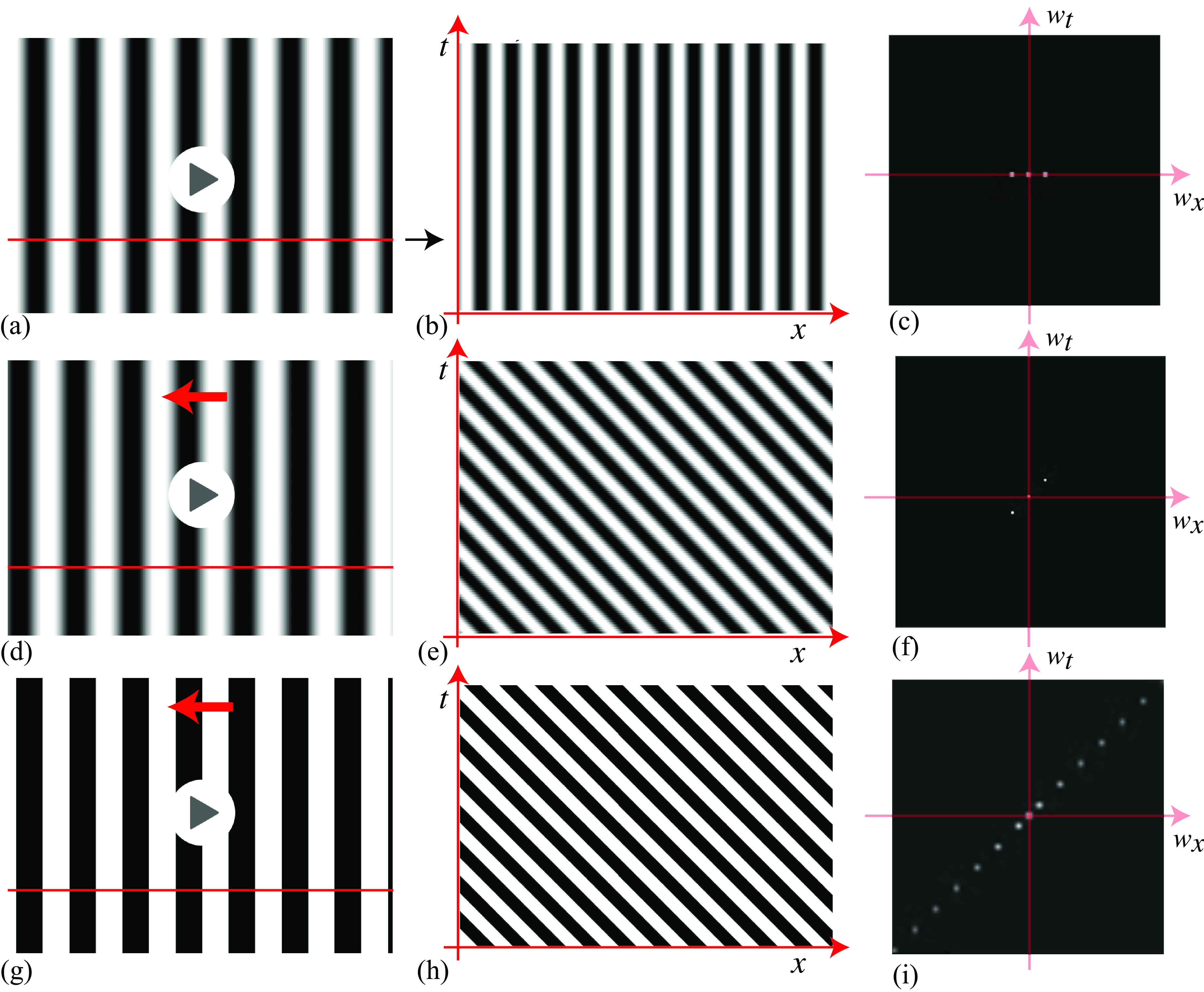
The signals, and magnitudes of their space-time Fourier transforms, are developed in Figure 46.6 and Figure 46.7, building-up from simpler signals. The three rows of Figure 46.6 show a stationary sinusoid, a moving sinusoid, and a moving square wave. The spatiotemporal Fourier transform of the stationary sinusoid, \(f(x,y,t) = \cos(\pi \omega x)\), is \((\delta(w_x + \omega) + \delta(w_x - \omega)) \delta(w_y) \delta(w_t)\). We have added a constant bias to the sinusoid to avoid negative intensity values, leading to an impulse at the center of the Fourier transform, as shown in Figure 46.6 (c). The resulting three colinear impulses are along the temporal frequency, \(w_t = 0\) line. A space-time plot of the signal (Figure 46.6[b]) shows only vertical structures, indicating no motion.
A moving sinusoid has a similar Fourier transform magnitude (Figure 46.6[f]) but with the spatiotemporal energies along a line perpendicular to the moving structures in the spatiotemporal signal (Figure 46.6[e]). A moving square wave is similar, but the extra harmonics needed to construct the square wave visible in the Fourier transform (Figure 46.6[i]).
Continuing the development of the illusion, Figure 46.7 [c] shows the Fourier transform and space-time plot of a square wave moving in 1/4 period jumps each time increment. This signal can be formed from Figure 46.6 (h) by applying a periodic sample-and-hold function, resulting in the spectrum of Figure 46.6 [i] replicated over temporal frequencies, and multiplied by a sinc function over temporal frequency. The resulting Fourier transform magnitude is shown in Figure 46.7 [c].

Because orientation in space-time tells motion direction (section Section 19.2 the space-time plot of Figure 46.7 [b] shows that the motion should be perceived to the left. This will be consistent with the behavior of velocity tuned filters (section Section 22.4.2) responding to the lowest spatiotemporal frequency impulses shown in Figure 46.7 [c]. However, if we remove the lowest spatial frequency sinusoid from the signal, the result is shown in Figure 46.7 [e], with spatiotemporal Fourier transform shown in Figure 46.7 [g]. Now the lowest spatiotemporal frequency cosine wave is oriented in the other direction. This opposite slope is also visible in the spatial domain, in the space-time plot of Figure 46.7 [e], and especially if we apply a low-pass filter, resulting in Figure 46.7 [f].
The signal of the second row of Figure 46.7 poses a conundrum. It can be argued that the signal moves to the left, just as does the signal of row 1 of Figure 46.7. The pattern match, that is, the minimum correlation signal indeed moves to the left. But the vision system examining the orientation of the lowest spatiotemporal frequency components of the signal in Figure 46.7 [g], or looking at the dominant orientations in the space-time plots of figures Figure 46.7 (e and g), would find a signal moving to the right! Videos showing each signal are available on the book’s web page. These illusions give support to the spatiotemporal energy models for human motion processing.
46.5 Concluding Remarks
In this section we have introduced a conceptually simple approach to compute the motion in sequences. But are the estimated patch displacements meaningful? Do they correspond in any way to the motion in the 3D world?
We have computed motion between two frames before really understanding the motion formation process (i.e., how a camera looking at a moving 3D scene produces two-dimensional [2D] sequences). How should the correct motion look? And what do we want to do with it? So, before we move into more sophisticated motion estimation algorithms, let’s revisit the image formation process and examine how motion on the image plane emerges from the perspective projection of a dynamic 3D scene into a moving camera.